Sumif With Two Conditions
October 22, 2002 - by Bill Jelen
Bill sent in this week's Excel question.
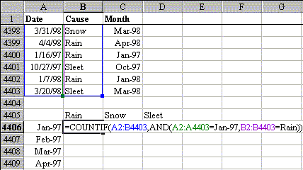
I have a database of events in Excel and my boss wants me to plot frequency charts by month. I read your trick to change daily dates to monthly dates and about Excel CSE formulas. I have tried every criteria I can think of in the Excel CountIf formula below to get it to look at 2 criteria.

Your situation could probably be solved easily with a pivot table (XL95-XL2000) or a pivot chart (XL2000 only). For now, let's address the question that you have asked. At the left is your worksheet. It looks like you will want to enter formulas in cells B4406:D4415 to calculate the number of certain events each month.
The CountIf function is a specialized form of an array formula which is great when you have a single criteria. It does not work well when you have multiple criteria. The following sample formulas would count the number of rows with Rain and the number of events in January 97:
=COUNTIF(B2:B4403,"=Rain")
=COUNTIF(A2:A4403,"="&A4406)
There is no way using CountIf to get the intersection of two conditions.
For any reader who is not familiar with how to enter array formulas, I highly recommend reviewing Use CSE formulas to supercharge Excel.
Bill did not state it in his question, but I want to build a formula which he can enter just once in cell B4406 that can easily be copied to the other cells in his range. By using absolute and mixed references in the formula, you can save the hassle of entering a new formula for each intersection.
Here is a quick review of absolute, relative, and mixed formulas. Normally if you enter a formula like =SUM(A2:A4403) in D1 and then copy the formula to E2, your formula in E2 will change to =SUM(B3:C4403). This is a cool feature of worksheets called "relative addressing", but sometimes we do not want that to happen. In this case, we want every formula to refer to the range A2:B4403. As we copy the formula from cell to cell, it should always point to A2:B4403. While entering the formula, hit F4 once after entering the range, and your formula will change to =SUM($A$2:$A$4403). The dollar sign indicates that that portion of the reference will not change as you copy the formula. This is called absolute addressing. It is possible to lock only the column with the $ and allow the row to be relative. This is called a mixed reference and would be entered as =$A4406. To lock the row but allow the column to be relative, use =B$4405. As you enter a formula, use F4 to toggle among the four flavors of relative, absolute and mixed references.
Here is the formula for cell B4406:
=SUM(IF($C$2:$C$4403=$A4406,IF($B$2:$B$4403=B$4405,1,0),0))
Type the formula. When you finish the formula, hold down Ctrl, Shift and then enter. You can now copy the formula to C4406:D4406 and then copy those three cells down to each row in your result table.
The formula uses all three forms of mixed and absolute references. It nests 2 if statements since the AND() function did not seem to work in an array formula. For a better explanation of what is happening with the array functionality, re-read Use CSE formulas to supercharge Excel mentioned above.
