Pivot Table Tips
August 20, 2002 - by Bill Jelen
You probably know how to create a basic Excel pivot table. Here are some obscure Excel pivot table tricks which will help you get the most out of pivot tables. You will learn how to convert a data field to show percentage of the total and then how to ensure that the largest items appear first within each group.
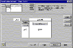
The Basics:
Select a cell in an Excel list, Choose Data > Pivot Tables, and Excel will walk you through the pivot table wizard. Here on step 3 of 4, you drag fields to the row, column, data, or page section of the pivot table.
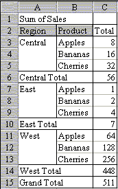
At right, you can see the familiar old basic default pivot table. Regions and products are sorted alphabetically, totals by region. But there is more available than this! The trick is to double click a field name when you are in Pivot Table Wizard step 3 of 4.
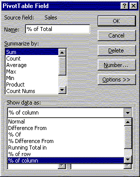
For example, if you drag the field Sales into the Data area twice, and double click on the second instance, you get the dialog box shown below left. By typing a new name in the Name field ("% of Total") and choosing % of Column from the "Show Data as" field, you can show both sales and the percent of total.
Then double click the Region field. On the next dialog, click the Advanced button and you will get the pivot table shown below right.
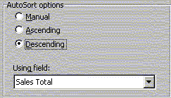
In this dialog, select that region should be descending based on the field Sales. Double click the product field and repeat the same process for the product field.
Not shown here, but in the same dialog box is an AutoShow Automatic field where you can specify that you want to see only the top/bottom x members of each group.
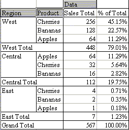
Shown at the right is our "jazzed up" pivot table. The West region is shown on top because they had the highest sales. Within each region, the products are ordered in descending sales order. It shows both Sales and % of Total Sales.
All of this was achieved with dialog boxes accessed from a few double clicks on the grey field names in the pivot table. So, the next time you need to create a pivot table, try double clicking the field name tiles to exert some extra control.
