Prevent Excel Duplicates
September 03, 2002 - by Bill Jelen
How in Excel can I make sure that duplicate invoice numbers are not entered in a particular Excel column?
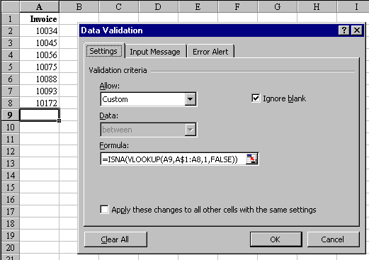
In Excel 97, you can use the new Data Validation feature to do this. In our example, the invoice numbers are being entered in column A. Here is how to set it up for a single cell:

- The next cell to be entered is A9. Click in cell A9, and select Data>Validation from the menu.
- In the "Allow:" drop down box, choose "Custom"
- Enter this formula exactly how it appears:
=ISNA(VLOOKUP(A9,A$1:A8,1,FALSE)) - Click the Error Alert tab in the Data Validation dialog box.
- Make sure that the "Show alert" box is checked.
- For Style:, pick Stop
- Enter a Title of "Non Unique Value"
- Enter a message of "You must enter a unique invoice number."
- Click "OK"
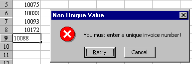
You can test it out. Enter a new value, say 10001 in cell A9. No problem. But, try to repeat a value, say 10088 and the following will appear:

The final thing to do is to copy this validation from cell A9 to the other cells in column A.
- Click in column A and select Edit>copy to copy the cell.
- Select a large range of cells in column A. Perhaps A10:A500.
- Select Edit, Paste Special. From the Paste Special dialog, select "Validation" and click OK. The validation rule that you entered from cell A9 will be copied into all of the cells down to A500.
If you click in cell A12 and pick Data Validation, you will see that Excel changed the validation formula to be =ISNA(VLOOKUP(A12,A$1:A11,1,FALSE)) That is all that you need to know to make it work. For those of you who want to know more, I will explain in English how the formula is working.
=ISNA(VLOOKUP(A9,A$1:A8,1,FALSE))
We are sitting in cell A9. We are telling the Vlookup function to take the value of the cell we just entered (A9) and to try to find a match in the cells that range from A$1 to A8. The next argument, the 1, tells Vlookup that when a match is found to tell us the data from the first column. Finally, the False in the vlookup says that we are only looking for exact matches. Here is trick #1: If the VLOOKUP finds a match, it will return a value. But, if it does not find a match, it will return the special value of "#N/A". Normally, these #N/A values are bad things, but in this case, we WANT an #N/A. If we get an #N/A, then you know that this new entry is unique and does not match anything above it. An easy way to test if a value is #N/A is to use the ISNA() function. If something inside the ISNA() evaluates to an #N/A, you get a TRUE. So, when they enter a new invoice number and it is not found in the list above the cell, the vlookup will return an #N/A, which will cause the ISNA() to be true.
The second bit of trickery is in the second argument for the Vlookup function. I was careful to specify A$1:A8. The dollar sign before the 1 tells Excel that when we copy this validation to other cells, it should always start looking in cell of the current column. This is called an absolute address. I was equally careful not to put a dollar sign before the 8 in A8. This is called a relative address and tells Excel that when we copy this address, it should stop looking in the cell just above the current cell. Then, when we copy the validation and look at the validation for cell A12, the second argument in the vlookup correctly shows A$1:A11.
There are two problems with this solution. First, it will not work in Excel 95. Second, the validations are only performed on cells that change. If you enter a unique value in cell A9, and then go back up and edit cell A6 to be the same value you entered in A9, the validation logic in A9 will not be invoked and you will end up with duplicate values in your worksheet.
The old-fashioned method used in Excel 95 will address both of these issues. In the old method, you would have the validation logic sitting in a temporary column B. To set this up, enter the following formula in cell B9: =ISNA(VLOOKUP(A9,A$1:A8,1,FALSE)) Copy this formula from B9. Paste it in cells B2:B500. Now, as you enter invoice numbers in column A, column B will show TRUE if the invoice is unique, and FALSE if it is not unique.
