using form controls to select colums from a data table to populate a graph

[Benjamin92]

Hi all, thank you in advance for your help. I've been working on an Excel project at work this past week, and am stumped. I'm looking for a way to use form controls from the developer tab to make 1 graph, but select different columns from a data chart to populate the graph.

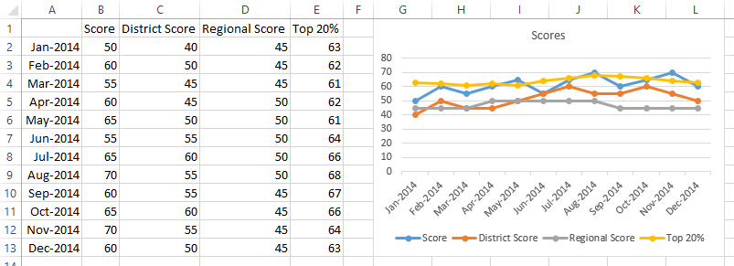
I have a data table with the following 5 column titles: 1. mm/yy 2. score 3. district score 4. regional score 5. top 20%.
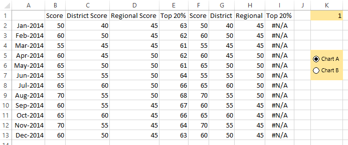
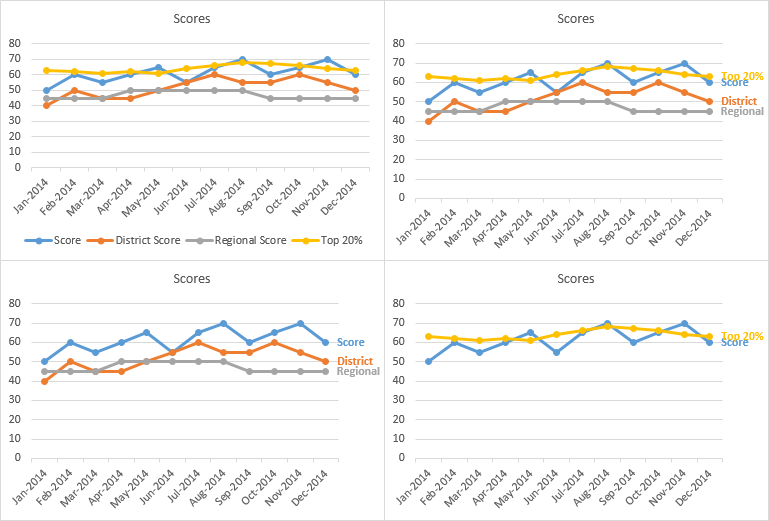
My goal is to use this data table to populate one graph, and use form controls to either select columns 1,2,3,and 4, or use columns 1,2,and 5 to populate the graph.

Any thoughts on the best way to do this?

Thank you!

 

[Jon Peltier]

Okay, here's how I would approach it. This is some dummy data I'm starting with and a chart of all of the series.

What I'm going to do is add some columns (F:I) that show or don't show data based on which of two option buttons is selected, and I'm going to make my chart from all of the data. When the values aren't shown in the worksheet, they will not appear in the chart.

Here's my new data range. At first the formula in cell F2 (and copied into the entire range F2:I13) is simply

=B2

I then add two option buttons and label them Chart A and B. I right click on one of them (doesn't matter which) and select Format Control, and on the Control tab, I click in the Cell Link box, and select cell K1. This cell tells me which of the buttons is selected, 1 or 2.

So I select A1:A13, then hold Ctrl while selecting F1:I13, and insert a line chart (below left). I delete the legend and instead label the last point in each series with the series name, and use label text that matches each series color (below right).

I keep the formulas in column F the way they are, since this series appears whichever option is selected. The formula in G2 (copied into G2:H13) is

=IF($K$1=1,C2,NA())

Which means show the value if the first option button is selected, or show #N/A instead. #N/A isn't plotted in a line or scatter plot.

Similarly in I2 (and filled into I2:I13) is this formula

=IF($K$1=2,E2,NA())

When the first option button is selected, I get Chart A (bottom left), and when the second is selected, I get Chart B (bottom right).

 

[Benjamin92]

Thank you for the step-by-step! It worked perfect and did exactly what I needed to do. Previously I had each graph mapped (one compared to district and region, one compared to top 20%), and was using an index,match function to pull the appropriate graph. The file size was way to big, and this shrunk it in half!

One more question, if you don't mind. Is there a way to hide the new tabs (F:I) without losing their function? When I hid them, they would no longer work to populate the graph.

Thank you!

 

[Jon Peltier]

You could stick the calculations in another sheet, and hide the sheet. Alternatively, you can hide the columns, and then you need to tell each chart to plot hidden cells:

Edit Data > Hidden and Empty Cells button (bottom left of dialog) > [X] Show data in hidden rows and columns.