How do i get this chart effect

Siyanna

Well-known Member
Joined
Nov 7, 2011
Messages
1,146
Hi

I have some data which gives me ydays score and todays score

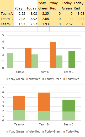
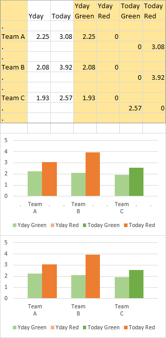
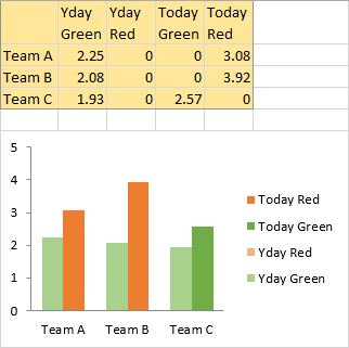
I want o show any figure that is greater than 3 in red else show it as green

So for each team i would need to 2 plots ydays score and todays score
Again depending on what the score was it will need to change colour
So side by side for each team i can see whether its in the Green or Red comparing both days

Here was my attempt

Yday RedYday GreenToday RedToday Green
TEAM A2.253.08
TEAM B2.083.92
TEAM C1.932.57


<colgroup><col><col><col><col><col></colgroup><tbody>
</tbody>

The formulas I used

=IF(D2>3,D2,"") - Copied down for yday red
=IF(D2<3,D2,"") - copied down for yday green
=IF(E2>3,E2,"") - copied down for today red
=IF(E2<3,E2,"") - copied down for today green

The formulas is there to show the values but struggling to get the Chart to actually show it side by side for both days to see what colour it was for yday and today

Hope that helps

Thanks
 

Excel Facts

When did Power Query debut in Excel?
Although it was an add-in in Excel 2010 & Excel 2013, Power Query became a part of Excel in 2016, in Data, Get & Transform Data.
Your formulas exclude the case where the score is exactly 3. Green occurs when the value is <3, red when it is >3. You should either make green <=3 or red >=3, or include a third condition for =3.

I set up my formulas as shown below, selected the shaded two-area range, and made a clustered column chart. That didn't work, so I made a stacked column chart. That also didn't work.

ConditionalClustered(Stacked)Columns1.png


What you need is a stacked and clustered column chart. This isn't built into Excel, but you can easily enough fake it.

I've staggered my data as shown below, where yesterday's and today's data are on different rows, and a blank row appears between categories (teams). From the shaded data I made a stacked column chart, and set the series gap width to zero. You don't see anything stacked, because one item of each stacked pair is always zero, but believe me, yesterday green is stacked on yesterday red, and the same for today green and red.

I put dots in the first column to help Excel plot the data correctly. The chart below is how it looks with the dots cleared after the plot is created.

ConditionalClustered(Stacked)Columns2.png


This still isn't perfect. The team names aren't centered under the clusters of columns. You can read my tutorial about Clustered and Stacked Column and Bar Charts to see how to make the chart above look better (below). Alternatively I've written Excel VBA software that makes this type of chart easily.

ConditionalClustered(Stacked)Columns3.png
 
Upvote 0
Hi

Firstly i want to say thank you so much

yes I completely missed the = 3 condition so i will need to add that and make that orange so yday orange and today orange

if i was to that - would the layout be totally different to the way you did it above?

Yes you are very right that the names are not centred..i could see the vba part or anything to centre it..Would i need some code to centre the names or would i need to fornat it differently to achieve this look?

Again thank you
 
Upvote 0
I did my charts using the appropriate formulas, so the layout is correct.

To see how to get centered labels, read the tutorial I cited in my earlier post.
 
Upvote 0

Forum statistics

Threads
1,212,933
Messages
6,110,751
Members
448,295
Latest member
Uzair Tahir Khan

We've detected that you are using an adblocker.

We have a great community of people providing Excel help here, but the hosting costs are enormous. You can help keep this site running by allowing ads on MrExcel.com.
Allow Ads at MrExcel

Which adblocker are you using?

Disable AdBlock

Follow these easy steps to disable AdBlock

1)Click on the icon in the browser’s toolbar.
2)Click on the icon in the browser’s toolbar.
2)Click on the "Pause on this site" option.
Go back

Disable AdBlock Plus

Follow these easy steps to disable AdBlock Plus

1)Click on the icon in the browser’s toolbar.
2)Click on the toggle to disable it for "mrexcel.com".
Go back

Disable uBlock Origin

Follow these easy steps to disable uBlock Origin

1)Click on the icon in the browser’s toolbar.
2)Click on the "Power" button.
3)Click on the "Refresh" button.
Go back

Disable uBlock

Follow these easy steps to disable uBlock

1)Click on the icon in the browser’s toolbar.
2)Click on the "Power" button.
3)Click on the "Refresh" button.
Go back
Back
Top