chart timestamped data, but need excel to "fill in" the times

[eric81]

Hello,
I have timestamped data of a door open/closed status. I only note the changes, so the data looks like this. 1 is open, 0 is closed.

7/23/2016, 10:10:34	1
7/23/2016, 10:10:38	0
7/23/2016, 10:10:39	1
7/23/2016, 10:10:40	0
7/23/2016, 10:11:41	1
7/23/2016, 10:11:42	0

<colgroup><col><col></colgroup><tbody>
</tbody>

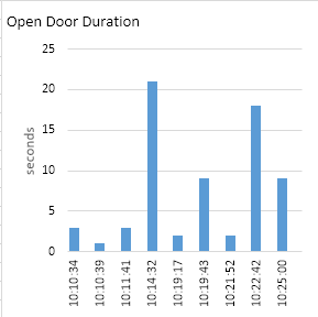
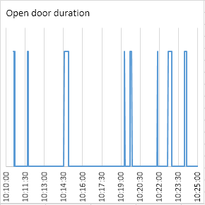
I want excel to generate a chart that lets me visualize the open/closed periods. I want to visually see how long the door is opened during the period. So I need excel to fill the y-value from one time stamp to the next change with the state. So from 10:10:34 to 10:10:37, I need excel to fill in 1's.

A line graph might work, but really anything that visulizes it would work. Bars, lines, whatever.

 

[thisoldman]

I think you'll find a column chart is easiest to read and is much less work.

Column Chart
I'm only posting a portion of the data I used for the chart; I expanded what you posted.

Excel 2012

	A	B	C	D	E	F
1	Date	Time	Open/Close			Duration
2	07/23/2016	10:10:34	1		10:10:34	3
3	07/23/2016	10:10:37	0
4	07/23/2016	10:10:39	1		10:10:39	1
5	07/23/2016	10:10:40	0
6	07/23/2016	10:11:41	1		10:11:41	3
7	07/23/2016	10:11:44	0
8	07/23/2016	10:14:32	1		10:14:32	21
9	07/23/2016	10:14:53	0

<colgroup><col style="width: 25pxpx"><col><col><col><col><col><col></colgroup><thead>
</thead><tbody>
</tbody>

Sheet1​

Worksheet Formulas Cell Formula E2 =IF(C2,B2,"") F2 =IF(C2,(B3-B2)*86400,"") <thead> </thead><tbody> </tbody>

<tbody>
</tbody>

Scatter chart
This is much more difficult for me to read.

Cell H2 was entered manually. The remainder of the column was populated by formula. Columns E and H were graphed.

Excel 2012

	A	B	C	D	E	F	G	H
1	Date	Time	Open/Close		Time	Start	End	Open
2	07/23/2016	10:10:34	1		10:10:34	1	0	1
3	07/23/2016	10:10:37	0		10:10:35	0	0	1
4	07/23/2016	10:10:39	1		10:10:36	0	0	1
5	07/23/2016	10:10:40	0		10:10:37	0	1	0
6	07/23/2016	10:11:41	1		10:10:38	0	0	0

<colgroup><col style="width: 25pxpx"><col><col><col><col><col><col><col><col></colgroup><thead>
</thead><tbody>
</tbody>

Sheet2​

Worksheet Formulas Cell Formula F2 =IFERROR(--(INDEX($C$2:$C$19,MATCH(E2,$B$2:$B$19,0))=1),0) G2 =IFERROR(--(INDEX($C$2:$C$19,MATCH(E2,$B$2:$B$19,0))=0),0) H3 =IF(F3=G3,H2,IF(F3,1,0)) <thead> </thead><tbody> </tbody>

<tbody>
</tbody>