Totals from 31 Daily Worksheets

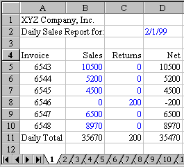
February 1999 Challenge: You have created a daily sales sheet in Excel. Each day, you paste a new worksheet into the workbook and give the sheet a name of 1 for Feb 1st, 2 for Feb 2nd, etc. At the end of the month, you have 28 sheets and want to total the sales, returns, and net sales for all 28 days on a new summary sheet. What is the fastest way to manage and enter this multi-sheet formula. To further complicate things, the total sales for each day may be on a different row. As always, better approaches to the problem as stated are acceptable.
Results
Fellow Excel tipster Ole P. Erlandsen offered an interesting twist. He suggested that you create sheets named 1-31. Reformat the sheet so that the totals are in row 4. Headings are in row 5. The data starts in Row 6 and extends down as far as necessary. The formula for B4 on each sheet is: =SUM(B5:B100). Then, on the summary sheet, you can add up the daily totals with this slick formula: =SUM('1:31'!B4). I love this formula - it allows you to add up a cell from each sheet in a workbook. This is an excellent tip.
Update! In 2006, David Gilbertson from Australia sent in this cool solution...
"Having just been introduced to the joys of a TV show dedicated to Excel, I was drawn to your site where I started by browsing through your past challenges. Feb '99 struck me as one that deserved a much simpler answer. If I was looking for my total sales (column B) for all 28 sheets, then the formula on the final tab would be =SUM('1:28'!B5:B65536)/2. And that's it. If you take a set of numbers and their total and add them all together, then divide by two, you get the total. 7 years and 2 months isn't that late, really."
Yes - this is a great trick - using the old accounting trick that I talked about in podcast 241.
Michael Beary & Jeff Borek both submitted an admirable macro to do the job.
Jason Szumlanski gets the nod as this month's winner for his formula which answered the question as stated. The original problem said that the daily sales total could be on any given line of a worksheet. Jason set up a workbook with 32 sheets. Sheets were named 1, 2, 3, 4, . . ., 31, and summary. On the summary sheet, Jason entered the numbers 1-31 in cells A5:A35. His formula for cell B5, to find the daily sales total from the 1st of the month is as follows:
=INDEX(INDIRECT("'"&$A5&"'!$A$1:$D$20"),MATCH("Daily Total", INDIRECT("'"&$A5&"'!$A$1:$A$20"),0),2)
The INDIRECT function says to take the text argument and to treat it as a reference to a range. Jason concatenates apostrophes around the value in cell A5 to cleverly point to a specific worksheet.
The MATCH function returns the relative position of the words "Daily Total" in a range.
The INDEX function takes three arguments: A range of cells, the row position you want within that range, and the column position. Jason uses the result of the MATCH function to indicate the ROW and then hardcodes 2 for the column.
Jason's answer relies on three seldom understood or used functions in Excel. Congratulations to Jason and thanks to Ole, Mike, Jeff and Jason for submitting answers to this month's challenge.
