
Recognize Your Top Sales Reps
October 10, 2005
To try this tip on your own computer, download and unzip CFH277.zip.
Are you responsible for managing a sales force? Build an Employee-Of-The-Day report to recognize and reward the best sales reps.
The computer system at work can probably produce a boring text report showing who sold what yesterday. I know a company that faxes this list out to each location and it is posted on the bulletin board in the back room. But – it is really just a boring list with 120 names listed in alphabetical order. No glory. No easy way to see who is doing the best.
We can use Excel to build this into a glitzy report recognizing the top five sellers from yesterday.
Here is the data in the current report. It lists the sales reps in no particular order with their sales figures from the previous day. This report is generated by your sales system and is placed on your server each day.

The above report will be overwritten each day by the sales system. So - start with a blank worksheet and build external link formulas to grab the current data from the sales worksheet. To build the formula shown below, you would follow these steps.
- Have the sales report open
- Open a blank workbook
- In cell B2, type an equals sign.
- Use the Window menu. Choose the sales report from the Window menu. In the sales report, use the mouse to touch cell B2. Excel will build a formula referring to $A$2. Type the F4 key three times to remove all of the dollar signs. Copy the formula from A2 down for many rows. You should copy it down far enough to cover your current sales reps plus more rows for future reps.
Repeat those steps in column C to build a formula to grab net sales.

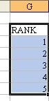
In column A, use the =RANK function to get the rank of this row's sales amongst all sales.

Note
The RANK function behaves strangely with ties. If there is a tie for 3rd place, both records will receive a 3. No record will receive a 4. While this is technically correct, this behavior will cause the VLOOKUPs to fail. Modify the formula shown above to be:
=RANK(C2,$C$2:$C$64)+COUNTIF(C$1:C1,C2)
Off to the Right, type the numbers 1 through 5.
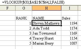
To the right of the numbers, use a VLOOKUP formula to return the sales rep name and sales.
Add a new worksheet. Use WordArt and ClipArt to make an attractive report. The formula in A9 is ="For "&Text(TODAY()-1,"mmmm d, yyyy"). Select cells C20:I20. From the menu, select Format - Cells - Alignment. Choose the option for Merge Cells. The formulas in C20:C24 point back to the worksheet range with the VLOOKUP formulas.

This attractive report can be hung daily in the employee bulletin board.