
Using Excel to Track Student Grades
October 06, 2006
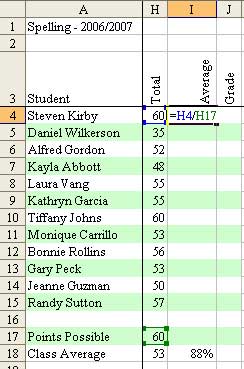
In today's episode, I talked about a simple gradebook application in Excel. Although the concept is simple, there are several formulas in the gradebook that can trip you up. The gradebook looks like this:

Vertical Headings
The headings in row 2 are turned on their side by using Format - Cells - Alignment. On the Alignment tab, change the orientation to 90 degrees.

Points Possible Row
It is important to have a row on the spreadsheet listing the total points possible for each assignment. Do not fill in the points possible for an assignment until you have entered the grades for that assignment. In the first figure above, the points possible are in row 17.
Total Formulas in Column H
Enter an =SUM function in H4 to total the scores for the first student. Copy this formula down column H for each student and for the points possible line. Excel automatically changes the relative references in the formula to point to the next row, etc.

Tricky: Average Formulas in Column I
The formula for I4 might seem like it would be simple. You might try entering =H4/H17, but this will cause a problem.
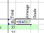
When you copy this formula down a few rows, it stops working. Here in row 6, the formula changed to =H6/H19. It is correct that Excel changed H4 to H6, but you want Excel to always absolutely pointing to H17 as the divisor in the calculation.

Go back and edit the formula in I4. You can select I4 and press F2, or simply double-click I4.
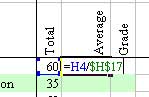
When the insertion point is right after the H17, press the F4 key. Excel inserts dollar signs to change H17 to $H$17.
The dollar sign before the H says that no matter which direction you copy the formula, you always want to point to column H.
The dollar sign before the 17 says that no matter which direction you copy the formula, you always want to point to row 17.
This is called an absolute reference.
When you copy this formula down to all students, Excel correctly always divides by the total points possible in row 17.

Converting Percentages to Letter Grades
You will use the VLOOKUP function to convert percentages to a letter grade. There are two ways to use the VLOOKUP function, and 90% of the time on this site, I use the version where Excel has to find an exact match in the lookup table. This version, however, uses the version of VLOOKUP where the table contains ranges of data.
In this version, the lookup table has to be sorted in low-to-high order. As you can see below, this requires you to take your school grading scale and turn it upside down. In the table below, row 4 is saying that any scores above a 0 will receive an F. Row 5 takes over and says that any scores above 65% will receive a D. In Row 6, anything at 69% or above is a D+. The basic idea is that Excel will find the number that is equal to or lower than the student's score.

-
To build the VLOOKUP in J4, start with
=VLOOKUP( -
The first argument is the student's score in
I4. -
The next argument is the range with your lookup table. In this example, the table is in
L4:M12. -
You want the formula to always point to this same range, so press the F4 key to change it to
$L$4:$M$12. -
The final argument is the column number from your table with the letter grade. In this example, it is a
2. -
The formula is
=VLOOKUP(I4,$L$4:$M$12,2).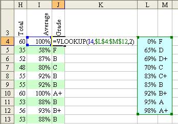
- Copy the formula down for all students.
The version that I used on the show is small - with few students and only a few assignments. You can download this smaller version to see how the formulas work. Right-click CFHGrades.zip.