
Pivot Tables in Excel 2007
February 25, 2007
Pivot tables improve in Excel 2007. On today's episode of Call For Help, I will show off the differences, plus some improvements that are only available in Excel 2007.
- To start, select one cell in your data. From the Insert ribbon, choose Pivot Table. Excel will display the new Create Pivot Table dialog.

- Assuming Excel selected the correct range for your data, click OK. Excel provides a blank pivot table on a new worksheet. You will notice that the Pivot Table Field List now has a list of fields at the top, and four drop zones at the bottom. Instead of dragging fields to the pivot table, you will drag fields to the drop zones at the bottom of the pivot table field list. The old "Page Fields" area is now called "Report Filter". The old "Data" area is now the " Σ Values" area.

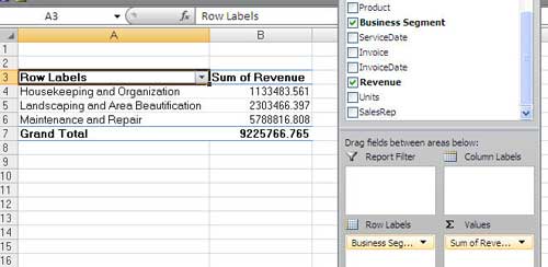
- If you checkmark a text field in the top of the pivot table field list, it will automatically jump to the Row Labels. If you checkmark a numeric field, it will automatically jump to the Σ Values section. Here is a pivot table after checking Business Segment and Revenue.
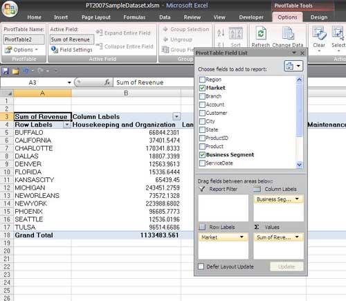
- It is easy to move a field by dragging it from one drop zone to another. In the next image, Business Segment is dragged to Column Labels. Market is added as a row label.
Formatting the Pivot Table
When your cell pointer is inside the pivot table, you will have two new ribbon tabs under the PivotTable Tools heading - Options and Design. On the Design ribbon, the PivotTable Styles gallery offers 85 built-in formats for pivot tables. It is not obvious, but the four option buttons for Row Headers, Column Headers, Banded Rows, and Banded Columns modify many of the 85 styles. Example: Turn on banded rows by clicking it's checkbox. Then, open the gallery, you will see that the previews for most of the 85 styles have changed.
By using combinations of the 4 checkboxes, you can easily access (2 X 2 X 2 X 2 X 85) 1,360 different styles for your pivot table. Don't forget that the 85 styles change if you choose any of the 20 themes on the Page Layout ribbon, so you have 27,200 different layouts available. If none of those work, you can access the New PivotTable Style… command at the bottom of the Pivot Table Styles gallery. (Creating a new style is a topic for another show - we only have 6 minutes!).In this image, I've turned on Row Headers, Column Headers, and Banded Rows and selected a dark orange layout. Note that Live Preview works in the gallery, You can hover over an item to see how it changes.

New Layout Options
In the next image, a pivot table has two fields in the Row section. Excel 2007 adopts a new layout called "Compact Form" as the default layout. Note that this layout jams both row fields into column A. You might like this layout, but I frequently visit the Report Layout dropdown on the Design ribbon to change back to the Outline Form.

New Filtering Options for Row & Column Fields
You have always been able to filter fields that were in the Page Area (uhhh, I mean Report Filter area). New in Excel 2007, you can apply filters to fields in the Row area. This is a pretty cool feature. In the next image, ServiceDate is in the row area. Hover over the words ServiceDate in the top of the PivotTable Field List and you will see a dropdown appear.

Open the dropdown. Choose Date Filters. The next flyout menu offers filters for This Week, Next Month, Last Quarter, and others. If you want to filter to a specific month or quarter, choose All Dates in Period and select a month or quarter from the final flyout menu.

All in all, pivot tables are easier to use in Excel 2007 and offer great new functionality. Mike Alexander and I have updated our best-selling Pivot Table Data Crunching Excel 2016 for Excel 2007.