
Finding Fraud with Excel
May 01, 2008
Forensic auditors can use Excel to quickly wade through hundreds of thousands of records to find suspicious transactions. In this segment, we will take a look at some of those methods.
Case 1:
Vendor Addresses vs. Employee Addresses
Use a MATCH function to compare the number portion of the street address of your employee records to the number portion of the street address of your vendors. Is there any chance some employees are also selling services to the company?
- Start with a list of vendors and a list of employees.
- A formula such as
=LEFT(B2,7)will isolate the numeric portion of the street address and the first few letters of the street name.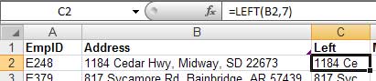
- Create a similar formula to isolate the same portion of the vendor addresses.
- The MATCH function will look for the address portion in C2 and try to find a match in the vendor portions in H2:H78. If a match is found, the result
will tell you the relative row number where the match is found. When no match is found, the #N/A will be returned.
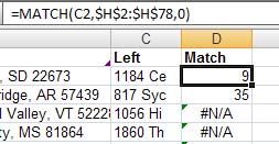
- Any results in the MATCH column which are not #N/A are potential situations where an employee is also billing the company as a vendor. Sort ascending by the MATCH column and any trouble records will appear at the top.
Case 2:
Unusual Swings in the Vendor Database
A company has 5000 vendors. We’ll use a scatter chart to visually find the 20 vendors who should be audited.
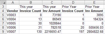
- Get a list of Vendor ID, Invoice Count, Total Invoice Amount for this year.
- Get a list of Vendor ID, Invoice Count, Total Invoice Amount for the previous year.
- Use VLOOKUP to match up these lists to five columns of data:
- Add new columns for Count Delta and Amount Delta:
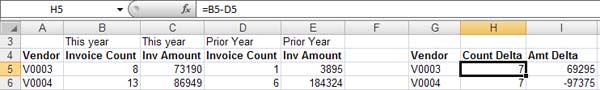
- Select the data in H5:G5000. Insert a scatter (XY) chart. Most of the results will be clumped in the middle. You are interested in the outliers. Start with the vendors in the boxed area; they sent fewer invoices for far more total dollars:
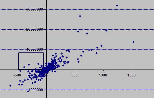
Note
To find the vendor associated with a point, hover over the point. Excel will tell you the count delta and amount delta to find in the original data set.
Case 3:
Using a Pivot Table to drill down
In this case, we take a look at invoices and receivables. Through various drill-downs of the data, discover which two accounts receivable analysts are spending Friday afternoons at the bar instead of working.
- I started with two data sets. The first is invoice data, Invoice, Date, Customer, Amount.
- The next data is Invoice, Receipt Date, Amount Received, A/R Rep Name
- Calculate a Days to Pay column. This is the Receipt Date - Invoice Date. Format the result as a number instead of a date.
- Calculate Day of the Week. This is
=TEXT(ReceiptDate,"dddd") - Choose one cell in the data set. Use Data - Pivot Table (Excel 97-2003) or Insert - PivotTable (Excel 2007)
- The first pivot table had Days To Pay down the size. Right-click one value and choose Group and Show Detail - Group. Group by 30 day buckets.
- Move Days to Pay to the column area. Put Customers in the Row area. Put Revenue in the Data area. You can now see which customers are slow to pay.
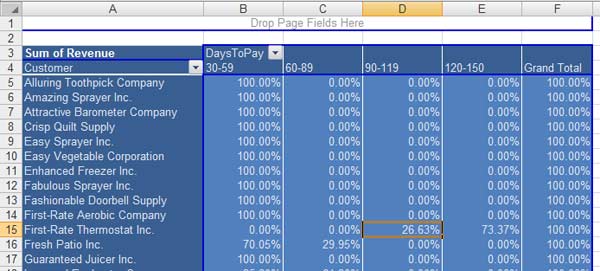
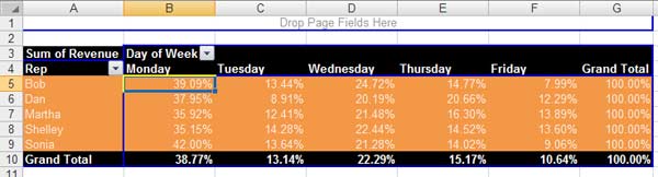
- Remove Days to Pay and put Weekday in the column area. Remove Customer and put Rep in the Row Area. You can now see the amounts received by day of the week.
- Choose a cell in the data area. Click the Field Settings button (in the pivot table toolbar in Excel 97-2003 or in the Options tab in Excel 2007).
- In Excel 97-2003 click More. In Excel 2007, click the Show Values As tab. Choose % of Row.
- The result: Bob and Sonia seem to process far less invoices on Friday than the others. Drop by their office on Friday afternoon to see if (a) they
are actually working, and (b) if there is a pile of unprocessed checks hanging out in their desk drawer until Friday.