(1) PIVOT TABLE NOT UPDATING (2) 2 TABLES PIVOT TABLE

[shah0101]

HI EXPERTS,

I HAVE TWO QUESTIONS:

1) MY TABLE IS UPDATING FINE BUT THE THE NUMBERS ON PIVOT TABLE NOT REFLECTING UPDATE (AFTER REFRESH). ANY SUGGESTIONS PLEASE?

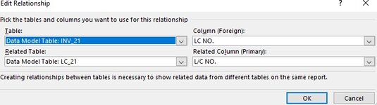
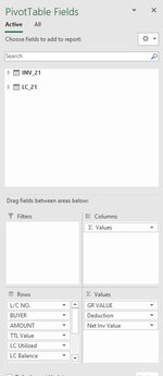
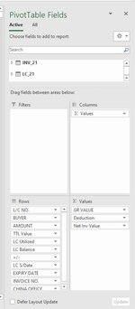
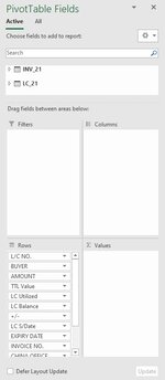
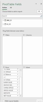
2) ON ANOTHER REPORT I HAVE TWO TABLES OUT WHICH I HAVE CREATED ONE PIVOT TABLE. THERE ARE COUPLE OF CALCULATED FIELDS AS WELL, RELATIONSHIP BETWEEN TABLES LOOKS GOOD (AS ATTACHED IMAGE), REFLECTING BALANCES JUST FINE AS REQUIRED BUT THE PROBLEM IS THAT THE PIVOT TABLE IS NOT BRINGING UP ENTRIES FROM THOSE ENTRIES WHICH ARE NOT YET RELATED IN THE SECOND TABLE. I WANT ALL ENTRIES TO BE IN THE PIVOT TABLE. IS IT POSSIBLE OR AM I ASKING TOO MUCH?

THANKS FOR THE HELP IN ADVANCE.

CHEER!

 

[Alex Blakenburg]

Is LC_21 Table2 ?

 

[shah0101]

Is LC_21 Table2 ?

Yes, please.

 

[Alex Blakenburg]

If you take the fields that appear in both tables from Table 2 (LC_21) and have
turned on "items with No Data on Row" then you should get all items from Table 2 even if they are not in Table 1.

Can you elaborate and or show me a picture of what this means.
"BUT THIS IS REPEATING ALL ENTRIES FOR TABLE 2 AGAINST EACH DIMENSION ON TABLE 1."
.

 

[shah0101]

If you take the fields that appear in both tables from Table 2 (LC_21) and have
turned on "items with No Data on Row" then you should get all items from Table 2 even if they are not in Table 1.

Can you elaborate and or show me a picture of what this means.
"BUT THIS IS REPEATING ALL ENTRIES FOR TABLE 2 AGAINST EACH DIMENSION ON TABLE 1."
.

Apologies for getting back late, I was not around.

To make the query simpler, instead of referring to tables as Table 1 and Table 2, I'll refer to their names:

Table 1: INV_21
Table 2: LC_21

LC_21 is the table which needs to bring all entries, but it is bringing only those entries against which relationship (One to Many) is found on "INV_21"
INV_21 is the table for which I need only those entries which corresponds to LC_21 but Pivot is bringing all entries
So basically it should work the other way around.

I have tried "items with No Data on Row" but what is does is against each LC_21 entry it is repeating all entries of INV_21 which is of no use.

I am not sure if I am still able to explain the problem.

Please advise.

Cheers!

 

[Alex Blakenburg]

I don't understand your pivot rows.
In rows I would expect to see.

• LC_21 > LC NO.
• LC_21 >Buyer

And the check box for "Show items with No Data on Row" should be ticked.

All the other items that are showing under rows seem to be values.

You are not showing giving me a full view of all the field names of both tables, so I am flying a bit blind here.
I assume all the other values under rows are coming from the INV_21 and this creating the multiplier effect that you don't want. Is this the case ?
Why do we have a values in the Row section ?

 

[shah0101]

I don't understand your pivot rows.
In rows I would expect to see.

• LC_21 > LC NO.
• LC_21 >Buyer

And the check box for "Show items with No Data on Row" should be ticked.

All the other items that are showing under rows seem to be values.

You are not showing giving me a full view of all the field names of both tables, so I am flying a bit blind here.
I assume all the other values under rows are coming from the INV_21 and this creating the multiplier effect that you don't want. Is this the case ?
Why do we have a values in the Row section ?

Please see attached is the full list of fields.

On Rows:
Yes, some of the fields like Amount, TTL Value, +/-, are value fields but I do no need the totals for that because these are simple fields brought up by Table: LC_21 without any calculation.

"LC Utilzied", is calculated field: =CALCULATE(sum(INV_21[NET VALUE]),FILTER(INV_21,INV_21[LC NO.]=LC_21[L/C NO.]))
"LC Balance", is calculated field: =LC_21[Sum of Total Available Value]-LC_21[LC Utilized]

And I do not need totals for these fields that is why we kept it in Rows.

"Invoice No." field is from "INV_21"


On Values:
All these are from "INV_21"



Please feel free to ask any questions you may have.

Looking forward to hear back.

 

[Alex Blakenburg]

I don't think you can do it they way you are trying to do it.
The "Show all Rows without data" is more aimed at giving you a summarised report that consistently shows all the categories for use in a Report or Chart.
This would involve having any values data that come from the fact table (INV_21) appear in the values section of the Pivot.

Having invoice no from the fact table, not to mention other value fields including calculated fields, is what is going to blow out your matrix.
(The Join between the Data Model tables is essentially a cross join)

I think your best bet to get what you want is most likely to use Power Query.

 

[shah0101]

I don't think you can do it they way you are trying to do it.
The "Show all Rows without data" is more aimed at giving you a summarised report that consistently shows all the categories for use in a Report or Chart.
This would involve having any values data that come from the fact table (INV_21) appear in the values section of the Pivot.

Having invoice no from the fact table, not to mention other value fields including calculated fields, is what is going to blow out your matrix.
(The Join between the Data Model tables is essentially a cross join)

I think your best bet to get what you want is most likely to use Power Query.

Thanks Alex,

Actually all the data in both tables is extracted from various different files through Power Query already but the problem is with Pivot to organize the data in such a way the required report is generated.

I also tried all fields in "Rows" but its not working either.

May be I am not good enough to explain it properly, let me elaborate it again what I am trying to achieve:

Table 2: LC_21 (Contains the Field"L/C NO." which is the key and have one to many relationship with "Table 1: INV_21". This
Table 1: INV_21 (Contains multiple or in some cases no entries related to "LC_21: L/C NO."

So all I want the Pivot to bring all entries from "LC_21" and their related entries in "INV_21". Can you please guide me how should I organize the fields to get the desirable result please?

Thanks in advance.

Cheers!

 

[Alex Blakenburg]

I also tried all fields in "Rows" but its not working either.

It is putting fields from INV_21 in "Rows" that is causing the issue in the first place.
I think your best chance of doing this particular report is to use Power Query. You can then easily ensure you get all the rows from the LC_21 table and you can control what appears on rows and what gets aggregated from the INV_21 table, without getting the Cross Join issue that you are experiencing using Pivots with the Data Model.

 

[shah0101]

It is putting fields from INV_21 in "Rows" that is causing the issue in the first place.
I think your best chance of doing this particular report is to use Power Query. You can then easily ensure you get all the rows from the LC_21 table and you can control what appears on rows and what gets aggregated from the INV_21 table, without getting the Cross Join issue that you are experiencing using Pivots with the Data Model.

I know it would be too much to ask but can you please please write me Power Query script please?