100% Stacked Bar Chart with % and Values

[DSL1970]

Hi All,


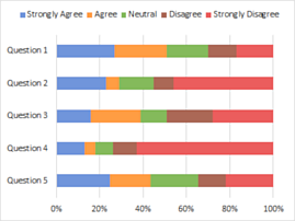
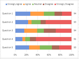
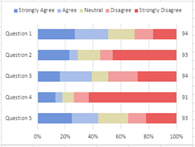
I haven't been able to find anything about this on the internet and curious if anyone can help me out with this issue I am having. I have been asked to pull together 15 questions with 5 responses Strongly Agree to Strongly Disagree as percentages in a 100% Stacked Bar Chart and a total number of respondents at the end of the 100% Stacked Bar Chart. How can I show the percentages in the charts (which I can do) and the value at the end? So in Q1 I have my chart with a 27% block for Strongly Agree through 17% for Strongly Disagree, then the Value of 94.

Like this https://exceljet.net/chart-type/100-stacked-bar-chart but with the value on the end (94 in Q1 based on the data set).

Data Set:

<colgroup><col span="2"><col><col><col span="2"><col><col></colgroup><tbody>
</tbody>

Strongly Agree Agree Neutral Disagree Strongly Disagree Grand Total % Grand Total Value
1 27% 24% 19% 13% 17% 100% 94
2 23% 6% 16% 9% 46% 100% 93
3 16% 23% 12% 21% 28% 100% 94
4 13% 5% 8% 11% 63% 100% 91
5 25% 19% 22% 13% 22% 100% 93
6 27% 24% 18% 10% 21% 100% 94
7 12% 15% 24% 18% 31% 100% 94
8 26% 16% 17% 14% 28% 100% 94
9 11% 11% 18% 24% 36% 100% 94
10 18% 15% 22% 19% 26% 100% 94
11 26% 12% 17% 20% 26% 100% 94
12 16% 4% 15% 19% 46% 100% 94
13 16% 11% 16% 26% 32% 100% 94
14 6% 4% 18% 26% 46% 100% 94
15 13% 7% 12% 20% 48% 100% 94


Regards,

D.

 

[thisoldman]

I'm working with five questions. Your data extends farther. My preference would be to have the Agrees to the right and the disagrees to the left, but I've continued with your ordering.

Organize thedata like this. H1 is deliberately left blank.

Book1
	A	B	C	D	E	F	G	H	I
1		Strongly Agree	Agree	Neutral	Disagree	Strongly Disagree			Label
2	Question 1	27%	24%	19%	13%	17%		94	0
3	Question 2	23%	6%	16%	9%	46%		93	0
4	Question 3	16%	23%	12%	21%	28%		94	0
5	Question 4	13%	5%	8%	11%	63%		91	0
6	Question 5	25%	19%	22%	13%	22%		93	0
Sheet1

Select the data from A1 to last of data in column F. Insert a 100% Bar chart.

With the Vertical axis selected, go to the chart format pane and check the box for "Categories in reverse order". Under "Horizontal axis crosses", select "At maximum value".

Move the legend to the top.

In the worksheet select H1 through the end of the data in column I. Press Ctrl+c to copy. Select the chart. Go to the home tab, click on the arrow beneath the large Paste icon and select "Paste Special...". In the popup, select "New series", "Columns", "Series Names in First Row", and "Categories (X Labels) in First Column". Click Ok.

There are several ways you can now move the new "Labels" Series to the secondary axis. I usually right-click on the chart and choose "Change Chart Type...". Scroll down in the bottom pane of the pop-up and check the box for Secondary axis in the "Labels" series row. Click OK. A new axis appears at the top of the chart.

Click the Plus icon next to the chart, and click on the small right-pointing arrow next in the "Axes" line. In this new sub-menu, check "Secondary Vertical" and uncheck "Secondary Horizontal". Change this new Vertical axis to "Categories in reverse order."

Click on the legend, click on the "Labels" entry in the legend to select it and press Delete.

Finish formatting as you please.

 

[DSL1970]

I'm working with five questions. Your data extends farther. My preference would be to have the Agrees to the right and the disagrees to the left, but I've continued with your ordering.

Organize thedata like this. H1 is deliberately left blank.

	A	B	C	D	E	F	G	H	I
1		Strongly Agree	Agree	Neutral	Disagree	Strongly Disagree			Label
2	Question 1	27%	24%	19%	13%	17%		94	0
3	Question 2	23%	6%	16%	9%	46%		93	0
4	Question 3	16%	23%	12%	21%	28%		94	0
5	Question 4	13%	5%	8%	11%	63%		91	0
6	Question 5	25%	19%	22%	13%	22%		93	0

<colgroup><col><col><col><col><col><col><col><col><col><col></colgroup><thead>
</thead><tbody>
</tbody>

Sheet1​

Select the data from A1 to last of data in column F. Insert a 100% Bar chart.

With the Vertical axis selected, go to the chart format pane and check the box for "Categories in reverse order". Under "Horizontal axis crosses", select "At maximum value".

Move the legend to the top.

In the worksheet select H1 through the end of the data in column I. Press Ctrl+c to copy. Select the chart. Go to the home tab, click on the arrow beneath the large Paste icon and select "Paste Special...". In the popup, select "New series", "Columns", "Series Names in First Row", and "Categories (X Labels) in First Column". Click Ok.

There are several ways you can now move the new "Labels" Series to the secondary axis. I usually right-click on the chart and choose "Change Chart Type...". Scroll down in the bottom pane of the pop-up and check the box for Secondary axis in the "Labels" series row. Click OK. A new axis appears at the top of the chart.

Click the Plus icon next to the chart, and click on the small right-pointing arrow next in the "Axes" line. In this new sub-menu, check "Secondary Vertical" and uncheck "Secondary Horizontal". Change this new Vertical axis to "Categories in reverse order."

Click on the legend, click on the "Labels" entry in the legend to select it and press Delete.

Finish formatting as you please.

Thank you thisoldman - looks like you have put some work into this - I am using Excel 2016 and don't appear to have some of these options, but I will keep playing with it....

My change chart type doesn't have any secondary options and my paste special only gives me a bitmap option!

 

[thisoldman]

It was made in Excel 2016. The options that I described have been there since Excel 2013. How can I help you find them?

Here's a link to my working file: https://www.dropbox.com/s/ps595xmlpzzcxed/bar_chart_dsl1970.xlsx?dl=0

 

[DSL1970]

I think I have I now - Thanks!