3 Color Scale Conditinal Format

[eddecaso]

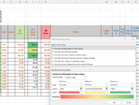
What am I doing wrong in trying to get I8 thru I1 to fill highlight in green if Column I is > Column G, in red if Column I is lower than Column K and in yellow if Volumn I is in midpoint/average of Columns G and K? I thin it works when I do for just one row but when I copy down the formats it doesn't work. And if I try to change Low, Mid, High criterias to a relative formula it doesn't allow me.

 

[awoohaw]

This is not 3 scale, imnot sure how important the scale is for midpoint values:

mr excel questions 12.xlsm
	G		I	J	K	L	M
1	BA Price		Current Price	BB Price	Green	Red	Yello
2	13.30		13.23	13.11	FALSE	FALSE	TRUE
3	12.80		12.76	12.64	=I2>G2	=I2<J2	=AND(I2<=G2,I2>=J2)
4	14.68		14.73	14.51	TRUE	FALSE	FALSE
5	12.64		12.54	12.47	FALSE	FALSE	TRUE
6	13.01		12.75	12.84	FALSE	TRUE	FALSE
7	13.74		13.62	13.56	FALSE	FALSE	TRUE
8	12.20		11.95	12.06	FALSE	TRUE	FALSE
9	14.35		14.22	14.15	FALSE	FALSE	TRUE
10	13.50		13.38	13.34	FALSE	FALSE	TRUE
11	12.27		12.23	12.14	FALSE	FALSE	TRUE
Sheet31

Cell Formulas
Range	Formula
K2,K4:K11	K2	=I2>G2
L2,L4:L11	L2	=I2<J2
M2,M4:M11	M2	=AND(I2<=G2,I2>=J2)
K3:M3	K3	=FORMULATEXT(K2)

Cells with Conditional Formatting
Cell	Condition		Cell Format	Stop If True
I2:I11	Expression	=I2<J2	text	NO
I2:I11	Expression	=AND(I2<=G2,I2>=J2)	text	NO
I2:I11	Expression	=I2>G2	text	NO

 

[awoohaw]

here it is with five colors so you can see the ranges between extremes and average:

mr excel questions 12.xlsm
	G		I	J
1	BA Price		Current Price	BB Price
2	13.30		13.23	13.11
3	12.80		12.72	12.64
4	14.68		14.73	14.51
5	12.64		12.54	12.47
6	13.01		12.75	12.84
7	13.74		13.65	13.56
8	12.20		11.95	12.06
9	14.35		14.22	14.15
10	13.50		13.38	13.34
11	12.27		12.23	12.14
Sheet31

Cells with Conditional Formatting
Cell	Condition		Cell Format	Stop If True
I2:I11	Expression	=I2<J2	text	YES
I2:I11	Expression	=I2>G2	text	YES
I2:I11	Expression	=ROUND(I2,2)=ROUND(AVERAGE(G2,J2),2)	text	YES
I2:I11	Expression	=I2<AVERAGE(G2,J2)	text	NO
I2:I11	Expression	=AND(I2>AVERAGE(G2,J2),I2<G2)	text	NO

 

[eddecaso]

Thanks for you prompt reply Awoohaw. I think you meant row 8 when u said 2, Col G and Col K when u said U.

I believe it may be know working and if not I will tweek your formulas if I'm not understanding properly. Here are the cells after your suggestion