A VBA Slap on the Head Please!

bc4240

Board Regular
Joined
Aug 4, 2009
Messages
134
Office Version
  1. 365
Platform
  1. Windows
Been trying to figure this out on my own for two days and I just suck!! Should be simple for someone. Got some Contextures code and have modified it some. Here's the jist.....

1) The top of the VBA code works like a charm, calling a set of Combo boxes (tempCombo & tempCombo2) into column B and column C cells that contain "data validation". I am using combo boxes because the dang font size is way too small to be seen in an excel data validation drop down list at lower window magnification (excel should give options for this on going issue....arrg anyway!!!!)
2) B7:C18 all have data validation.
3) Cells B7:B18 call on are Name Defined as "Animal".
4) Cells C7:C18 have a "dependent" formula in the data validation formula bar like this: =INDIRECT($B7&"x"). This formula takes the chosen value from the B cell (dog, cat, birds, elephant) and adds an "x" to the word e.g. dogx
5) dogx, birdsx etc. are defined names for the various type of birds, dogs etc. If I choose dog in B7 then C7 should populate with a list "boxer, lab, retriever, poodle, pug. But ALAS nothing but A$$, my code has failed me (observe):

Thanks for any help provided in adavance.

VBA Code:
Private Sub Worksheet_SelectionChange(ByVal Target As Range)
    Dim str As String
    Dim cboTemp As OLEObject
    Dim ws As Worksheet
    Set ws = ActiveSheet
    
    On Error Resume Next
    If tempCombo.Visible = True Then
        With tempCombo
            .Top = 10
            .Left = 10
            .ListFillRange = ""
            .LinkedCell = ""
            .Visible = False
            .Value = ""
        End With
    End If
    
    If tempCombo2.Visible = True Then
        With tempCombo2
            .Top = 10
            .Left = 10
            .Visible = False
            .LinkedCell = ""
            .Value = ""
        End With
    End If
   
        
    On Error GoTo errHandler
    If Target.Count > 1 Then GoTo exitHandler
    
    'the following segment of code insures that the correct combo box is used in the correct column (left column vs. right column)
    On Error GoTo errHandler
    If (Target.Column = 3 Or Target.Column = 2) And (Target.Validation.Type = 3) Then
        If Target.Column = 2 Then
            Set cboTemp = ws.OLEObjects("TempCombo2")
        ElseIf Target.Column = 3 Then
            Set cboTemp = ws.OLEObjects("TempCombo")
        Else
            Exit Sub
        End If
         
        With cboTemp
            'the following code inserts the combo boxes into the cells containing cell validation only
            .LinkedCell = Target.Address
            .Visible = True
            .Left = Target.Left
            .Top = Target.Top
            .Width = Target.Width + 3
            .Height = Target.Height + 5
            If Target.Column = 3 Then
                .ListFillRange = Cells(Target.Row, Target.Column - 1)
            End If
            
            .ListFillRange = ws.Range(str).Address
            If .ListFillRange <> str Then
        'for dynamic named ranges
        str = Target.Validation.Formula1
        str = Right(str, Len(str) - 1)
        Set wb = ActiveWorkbook
        Set nm = wb.Names(str)
        Set wsNm = wb.Worksheets _
          (nm.RefersToRange.Parent.Name)
        Set Rng = wsNm.Range _
          (nm.RefersToRange.Address)
        .ListFillRange = "=INDIRECT($B8 & ""x"")"
      End If
           
           End With
           cboTemp.Activate
    End If
             
   On Error GoTo errHandler
   If Target.Count > 1 Then GoTo exitHandler
          
exitHandler:
  Application.ScreenUpdating = True
  Application.EnableEvents = True
  Exit Sub
errHandler:
  Resume exitHandler
End Sub

Combo 1.png
Combo 2.png
[/SIZE]
 
Last edited by a moderator:

Excel Facts

Remove leading & trailing spaces
Save as CSV to remove all leading and trailing spaces. It is faster than using TRIM().
OK looks like I have to answer my own question here. Did some digging back though an old project and realized I had a solution to this. So for all of you who are looking for a way to add Dependent Combo Boxes to cells to magnify the list within, here we go!!

1. You need to make a data table consisting of columns like this:
Tables.png

this data can be wherever you'd like it, on your Active Worksheet in some out of the way columns, or on another Worksheet hidden away.

2. "Animal" is the list I will load into my #1 Combo Box (ironically named tempCombo2). Each of the names in the "Animal" list, as you can see, are the names of the column headers that are other lists. List of that type of animal.

3. After I choose an animal in my #1 Combo Box (tempCombo2) I want to click on my #2 Combo Box (named tempCombo) and see that animal's types loaded there.

4. We need to count how many names are in each of the above list for an OFFSET cell function we will need later. So in the cell above "Animal" (where you see the number 4) put this function: =COUNTIF(F3:F20,"?*") This will count the number of items in the "Animal" list. Do the same for every other list (dog, birds, etc.). You can just copy and then paste the function above each of the other lists if you'd like.

5. Now we need to name every list. So go to Formulas> Name Manager and New and you'll see a box like this pop up:
Name Manager.png

Where it says Name: type in Animal and where it says Refers to: type in this function: =OFFSET(Sheet1!$F$3,0,0,Sheet1!$F$1 +1,1) Click OK. If you'll notice, this offset function is defining the location and height of the list we are naming Animal. But also the name Animal can now be used as a function based package in other places in Excel. (Show you in a minute). The Sheet1! name will change depending on what you named your Worksheet. If you just click on the first entry in your list under "Animal" it will fill the correct Sheet name and cell location for you. The same is true for the next part of the function Sheet1!$F$1, just click in the cell where our =COUNTIF(F3:F20,"?*") function is located and it will fill in the Sheet name and cell location for you.

Now do this same thing for each of the other lists using the corresponding name dog, birds, cat, elephant. The =OFFSET(Sheet1!$F$3,0,0,Sheet1!$F$1 +1,1) Sheet name and cell locations will change for each OFFSET function.

6. Now when you return to your Name Manager window after your last named list is completed it should look like this:
Name Manager2.png


7. Now go to where you'd like to have your Combo Boxes and create a field of two columns (for this example I am using columns B and C)and make those columns have as many rows as you need. We need to assign a color to this area for VBA coding purposes (ahead). I have chosen the color vb ColorIndex 19. Looks like so:

Sheet.png


8. Go to the Developer tab (don't have it?? you need to get it. There are a lot of tutorials on that, so go search). Once you have it click Developer>Design Mode and Insert. Should look like this:
Developer.png


9. Choose Active X and Combo Box (2nd from Left top row). Draw two Combo Boxes (mine are colored green above). Doesn't matter where you put them but I'd at least put the one that will be your left box to the left and the one that'll be your right box on the right. They both will be invisible once the VBA code begins and will not show up until you call them by clicking in one of the colored cells you have designated for them to display in.

10. Now let make sure each of the Combo Boxes is named correctly so the VBA code will recognize them and make sure all the other properties are correctly assigned. So right click on the left box and and choose Properties. In the name area rename it tempCombo2 and fill each area of the properties box like this: (pay close attention to ListFillRange Type in "Animal" hit ENTER). Now we have used one of our Defined Names to deliver information through the Properties Box back to the VBA code for its use. (groovy man groovy!!) The VBA code ahead will do all the rest.
Combo1.png


As a reminder when you type new information in the areas above hit ENTER to insure the change has been enforced.

Do the same for Combo Box 2 on the right naming it tempCombo:
Combo 2.png


Once both Properties Boxes have been updated, use the X in the upper right hand corner of the Properties Box to close it.

11. Your Design mode button should still be activated. Now click on the "View Code" button. A VBA Project window will open. It should look like this:

VBA Code Manager.png


Double click your active sheet mine in this example is Sheet1. Then copy and paste this VBA code into the white open area to the right:

VBA Code:
Private Sub Worksheet_SelectionChange(ByVal Target As Range)
    Dim str As String
    Dim cboTemp As OLEObject
    Dim ws As Worksheet
    Set ws = ActiveSheet
    
  'This sets the size and shape of the "Animal Type" Combo Box (#2 Combo Box) when it is visible, but makes it invisible until the cell where it will be attached is clicked.
    On Error Resume Next
    If tempCombo.Visible = True Then
        With tempCombo
            .Top = 10
            .Left = 10
            .ListFillRange = ""
            .LinkedCell = ""
            .Visible = False
            .Value = ""
        End With
    End If
    
'This sets the size and shape of the "Animal" Combo Box (#1 Combo Box) when it is visible, but makes it invisible until the cell where it will be attached is clicked.
    If tempCombo2.Visible = True Then
        With tempCombo2
            .Top = 10
            .Left = 10
            .Visible = False
            .LinkedCell = ""
            .Value = ""
        End With
    End If
  
'If there is an error nothing will happen (nothing works).
    On Error GoTo errHandler
    If Target.Count > 1 Then GoTo exitHandler
    
'The following segment of code insures that the correct combo box (tempCombo vs. tempCombo2) is used in the correct column (left column vs. right column). It also demands that the Combo Boxes only appear in cells with a designated color (in this case vb ColorIndex 19 (yellow gold). If the color is changed the code must be changed to match the color.
        
        On Error GoTo errHandler
    If (Target.Column = 2 Or Target.Column = 3) And (Target.Interior.ColorIndex = 19) Then
        If Target.Column = 2 Then
            Set cboTemp = ws.OLEObjects("TempCombo2")
        ElseIf Target.Column = 3 Then
            Set cboTemp = ws.OLEObjects("TempCombo")
        Else
            Exit Sub
    End If

 'This part of the code insures that the tempCombo Box (#2 Combo Box) has it's ListFill Range populated with the lists of words (names) associated with the tempCombo2 value, e.g. dog = lab, retriever, etc..
        
        With cboTemp

            .LinkedCell = Target.Address
            .Visible = True
            .Left = Target.Left
            .Top = Target.Top
            .Width = Target.Width + 18
            .Height = Target.Height + 5
            
            If Target.Column = 3 Then
                .ListFillRange = Cells(Target.Row, Target.Column - 1)
            End If

          
           End With
           cboTemp.Activate
    
    End If

    
'This part of the code allows the actions above to continue if correct, or stop the code from working if incorrect.
    
exitHandler:
  Application.ScreenUpdating = True
  Application.EnableEvents = True
  Exit Sub
errHandler:
  Resume exitHandler
End Sub


It should look like this:
VBA Code Manager Full.png


All of the writing in green in the code give a little explanation of what each section of the code is doing.

12. Click the Save icon under Edit tab on the VBA Project Editor, then choose the File tab and choose "Close and Return to Excel". Next click on the Design Mode button turning it off. Finally click on any blank cell. You Combo Boxes should disappear.

13. At LAST!!! Click on one of the left colored cells. Your tempCombo2 Box should appear choose an animal from the dropdown lists. Now click on the colored cell to the right....your tempCombo Box should appear and it should have the list of animals corresponding to which ever animal you chose to the left. Only the colored cells will show the Combo Boxes!!
Final.png


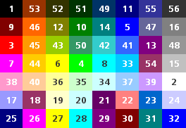
14. Don't like that color. The you can change it. You have 56 other VBA color's to choose from. Go back into the VBA code and look for this line,

If (Target.Column = 2 Or Target.Column = 3) And (Target.Interior.ColorIndex = 19) Then

Go to this sight and look up the RGB or HEX value of the color you like. Change your cells to match that color (remember the ColorIndex number) and replace 19 above with the new color number that matches your cells.


15. At this point if something doesn't work it's your color not matching or your Properties for your Combo Boxes losing the "Animal" out of the ListFillRange area. Go back and look and fix it from there. Good luck :) Don't call me :0

ENJOY!!!!!
 
Upvote 0
Solution
Oh Sorry I forgot to key you in on the most important part, enlarging you text inside the Combo Box Dropdown. Just go to the Properties Box for each Combo Box and go to "Font". Click on the area where the font name is and select the drop arrow this will open up a control box so that you can change the font characteristics. Now I'm done ;)
 
Upvote 0
Hello, I saw your example and got me thinking about something!

VBA Code:
If Target.Column = 3 Then
                .ListFillRange = Cells(Target.Row, Target.Column - 1)
            End If

Is this part responsible for populating the drop down list on the combo box? How does it work? In my mind this only selects a given cell?

I'm tryin a similar code but for other purpose and I'm having trouble to get to work a OFFSET function on the Source option of a data validation field into filling the combo box within VBA code...
 
Upvote 0
ListFillRange is a string, so it's using the value in that cell as the name/address of the source range, not using that one cell as the source.
 
Upvote 0

Forum statistics

Threads
1,214,625
Messages
6,120,598
Members
448,973
Latest member
ksonnia

We've detected that you are using an adblocker.

We have a great community of people providing Excel help here, but the hosting costs are enormous. You can help keep this site running by allowing ads on MrExcel.com.
Allow Ads at MrExcel

Which adblocker are you using?

Disable AdBlock

Follow these easy steps to disable AdBlock

1)Click on the icon in the browser’s toolbar.
2)Click on the icon in the browser’s toolbar.
2)Click on the "Pause on this site" option.
Go back

Disable AdBlock Plus

Follow these easy steps to disable AdBlock Plus

1)Click on the icon in the browser’s toolbar.
2)Click on the toggle to disable it for "mrexcel.com".
Go back

Disable uBlock Origin

Follow these easy steps to disable uBlock Origin

1)Click on the icon in the browser’s toolbar.
2)Click on the "Power" button.
3)Click on the "Refresh" button.
Go back

Disable uBlock

Follow these easy steps to disable uBlock

1)Click on the icon in the browser’s toolbar.
2)Click on the "Power" button.
3)Click on the "Refresh" button.
Go back
Back
Top