Add New Variable to Shapes

Doflamingo · Sep 3, 2019

Hi all,

Here is the code to create a structure chart from range A to range C of the sheet ‘’BD’’

Here is a screenshot of the sheet ‘’BD’’
https://www.dropbox.com/s/vyik32v24dp2ysm/sheet BD.png?dl=0

There is the ‘’Big father‘’ in A2 which is the ‘’Boss’’

The column B states all the ‘’sub father’’ with their ‘’children’’ that are in the column A except for the value ‘’Boss’’

For example the ‘’Boss’’ in cell A2 is the father of ‘’Vice President’’ in cell A3 that is the father of ‘’Employee13’’ in cell A11

The column C of the sheet ‘’BD’’ is the description of what you see inside the shapes in the sheet ‘’Shapes’’ where the structure chart is displayed once the macro is activated

Here is a screenshot of the sheet ‘’Shapes’’ of what I have currently with the data of the sheet ''BD''

https://www.dropbox.com/s/9p4pm5ukdmyly8h/Sheet Shapes.png?dl=0

Here is the code I have to display the structure chart in the sheet ''Shapes''

Code:

Sub créeShape(parent, niv, Attribut, coul) ' procédure récursive
  hauteurshape = 48
  largeurshape = 85
  colonne = colonne + 1
  forga.Shapes.AddShape(msoShapeFlowchartAlternateProcess, 10, 10, largeurshape, hauteurshape).Name = parent
  forga.Shapes(parent).Line.ForeColor.SchemeColor = 1
  txt = parent & vbLf & Attribut
  With forga.Shapes(parent)
    .TextFrame.Characters.Text = txt
    .TextFrame.Characters(Start:=1, Length:=1000).Font.Size = 8
    .TextFrame.Characters(Start:=1, Length:=1000).Font.ColorIndex = 0
    .TextFrame.Characters(Start:=1, Length:=Len(parent)).Font.Bold = True
    .TextFrame.Characters(Start:=1, Length:=Len(parent)).Font.ColorIndex = 3
    .Fill.ForeColor.RGB = coul
  End With
  forga.Shapes(parent).Left = débutOrg.Left + inth * colonne
  forga.Shapes(parent).Top = débutOrg.Top + intv * (niv - 1)
  For i = 1 To n
    If Tbl(i, 1) = parent And niv > 1 Then
      shapePère = Tbl(i, 2)
      
      forga.Shapes.AddConnector(msoConnectorElbow, 100, 100, 100, 100).Name = parent & "c"
      
      forga.Shapes(parent & "c").Line.ForeColor.SchemeColor = 22
      forga.Shapes(parent & "c").ConnectorFormat.BeginConnect forga.Shapes(shapePère), 3
      forga.Shapes(parent & "c").ConnectorFormat.EndConnect forga.Shapes(parent), 1
      
   End If
   
   If Tbl(i, 2) = parent Then créeShape Tbl(i, 1), niv + 1, Tbl(i, 3), f.Cells(i + 1, 1).Interior.Color
  Next i
  
End Sub

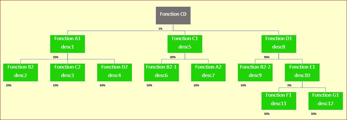
My problem is that I would like to expand my variables, I add a new range of variable in the column D of the sheet ‘’BD’’ and I would like that the specific variable be not included in the shapes like the variable of the column C are, but rather be below and at the left of the shapes they are related to.

Here a screenshot of what I would like to obtain
https://www.dropbox.com/s/emm9bkqm9eanmfm/goal.png?dl=0

I have changes the code above with the red lines that represent the values of the column D but that does not work

Code:

Sub créeShape(parent, niv, Attribut, coul) ' procédure récursive
  hauteurshape = 48
  largeurshape = 85
  colonne = colonne + 1
  forga.Shapes.AddShape(msoShapeFlowchartAlternateProcess, 10, 10, largeurshape, hauteurshape).Name = parent
  forga.Shapes(parent).Line.ForeColor.SchemeColor = 1
  txt = parent & vbLf & Attribut
  With forga.Shapes(parent)
    .TextFrame.Characters.Text = txt
    .TextFrame.Characters(Start:=1, Length:=1000).Font.Size = 8
    .TextFrame.Characters(Start:=1, Length:=1000).Font.ColorIndex = 0
    .TextFrame.Characters(Start:=1, Length:=Len(parent)).Font.Bold = True
    .TextFrame.Characters(Start:=1, Length:=Len(parent)).Font.ColorIndex = 3
    .Fill.ForeColor.RGB = coul
  End With
  forga.Shapes(parent).Left = débutOrg.Left + inth * colonne
  forga.Shapes(parent).Top = débutOrg.Top + intv * (niv - 1)
  For i = 1 To n
    If Tbl(i, 1) = parent And niv > 1 Then
      shapePère = Tbl(i, 2)
      
      forga.Shapes.AddConnector(msoConnectorElbow, 100, 100, 100, 100).Name = parent & "c"
      
      forga.Shapes(parent & "c").Line.ForeColor.SchemeColor = 22
      forga.Shapes(parent & "c").ConnectorFormat.BeginConnect forga.Shapes(shapePère), 3
      forga.Shapes(parent & "c").ConnectorFormat.EndConnect forga.Shapes(parent), 1
      
   End If
   
   If Tbl(i, 2) = parent Then créeShape Tbl(i, 1), niv + 1, Tbl(i, 3), f.Cells(i + 1, 1).Interior.Color
  Next i
  
[COLOR=#ff0000]  For u = 1 To n[/COLOR]
[COLOR=#ff0000]    If Tbl(u, 1) = parent And niv > 1 Then[/COLOR]
[COLOR=#ff0000]      shapePère = Tbl(u, 2)[/COLOR]
[COLOR=#ff0000]      [/COLOR]
[COLOR=#ff0000]      forga.Shapes.AddConnector(msoConnectorElbow, 100, 100, 100, 100).Name = parent & "d"[/COLOR]
[COLOR=#ff0000]      [/COLOR]
[COLOR=#ff0000]      forga.Shapes(parent & "d").Line.ForeColor.SchemeColor = 22[/COLOR]
[COLOR=#ff0000]      forga.Shapes(parent & "d").ConnectorFormat.BeginConnect forga.Shapes(shapePère), 3[/COLOR]
[COLOR=#ff0000]      forga.Shapes(parent & "d").ConnectorFormat.EndConnect forga.Shapes(parent), 1[/COLOR]
[COLOR=#ff0000]      [/COLOR]
[COLOR=#ff0000]   End If[/COLOR]
[COLOR=#ff0000]   [/COLOR]
[COLOR=#ff0000]   If Tbl(u, 2) = parent Then créeShape Tbl(u, 1), niv + 1, Tbl(u, 3), f.Cells(u + 1, 1).Interior.Color[/COLOR]
[COLOR=#ff0000]  Next u[/COLOR]
  
  
End Sub

Any idea ?

Doflamingo · Sep 30, 2019

Many thanks @Worf

I'm going to study the workbook provided, and I will let you know what I understand about it this week at the latest.

Many thanks for your help

Kind regards

Worf · Sep 30, 2019

You are welcome

I will wait for your feedback. There are at least two possible tasks ahead:

Converting your data table into mine.
Creating a chart that goes from bottom to top.

Doflamingo · Oct 5, 2019

Hello @Worf

I hope you are well !

As promised, I have worked on your macro. So It does not work on Excel 2016, but it works with Excel 2013 or 2010. It’s just slower with 2010 than with 2013

It works perfectly. My questions are:

Is it possible to get the data and the chart on the same page ? That would be great if the page was just the ‘’activesheet’’… so We should try Like you wrote it previously … converting my data table into yours.
What does represent the values in the column A in the sheet ‘’invoice’’ ?
What does represent the little blue shapes that appear at the top/left of the sheet ‘’object when the macro is activated ? Possible to remove it automatically ?
Is it possible to remove Code 1 and code 2 and use my own data instead ?
For the values entered in the sheet ‘’invoice’’ column M, is it possible they appear into the big shapes with the features ‘’bold’’ and ‘’calibri light
I tried to put some values in the column L of the sheet ‘’invoice’’ below ‘’Blank’’, But the values don’t appear into the big shapes. I would like those values appear into the big shapes below the values representing the ones entered in the sheet ‘’invoice’’ column

Many thanks in advance for what you have done until now, your help, time and kindness.

Kind regards

Worf · Oct 8, 2019

Hi

This is what I have so far:

Worf · Oct 8, 2019

This is the code; I will be back later to comment your questions…

Excel Workbook

A

B

C

D

1

Son

Father

Description

description 1

2

Fonction A1

Fonction C0

desc1

30%

3

Fonction B2

Fonction A1

desc2

20%

4

Fonction C2

Fonction A1

desc3

10%

5

Fonction D2

Fonction A1

desc4

60%

6

Fonction C1

Fonction C0

desc5

80%

7

Fonction B2-1

Fonction C1

desc6

50%

8

Fonction A2

Fonction C1

desc7

20%

9

Fonction D1

Fonction C0

desc8

90%

10

Fonction B2-2

Fonction D1

desc9

10%

11

Fonction E1

Fonction D1

desc10

0%

12

Fonction F1

Fonction E1

desc11

30%

13

Fonction G1

Fonction E1

desc12

30%

data2

Code:

Sub main()  ' run me
Adjust
CreateDiagram Sheets("object")
End Sub


Sub Adjust()
Dim lr%
Sheets("data2").Activate
[k:o].ClearContents
lr = Range("a" & Rows.Count).End(xlUp).Row
[k1] = "Seq": [L1] = "code1": [m1] = "code2"
[L2] = [b2]: [n1] = "info": [o1] = "info2"
[m2] = [b2]: [k2] = 2: [n2] = 0.01
[o2] = "desc0"
Range("a2:a" & lr).Copy [L3]
Range("b2:b" & lr).Copy [m3]
Range("c2:c" & lr).Copy [o3]
Range("d2:d" & lr).Copy [n3]
Range("k3:k" & lr + 1).Formula = "=row()"
End Sub


Sub CreateDiagram(Source As Worksheet)
Dim oSALayout As SmartArtLayout, QNode As SmartArtNode, QNodes As SmartArtNodes, oshp As Shape, Line%, _
i%, r As Range, PID$, mn, mx, ws As Worksheet, dt As Worksheet, crar(), c%, ad, v, t, s As ShapeRange
c = 1
ReDim crar(1 To c)
Set ws = Sheets("object"): Set dt = Sheets("data2")
ws.Activate
ws.[a:f].ClearContents
dt.[k1].CurrentRegion.Copy ws.[a1]
For i = 1 To ws.Shapes.Count
    ws.Shapes(1).Delete
Next
Set oSALayout = Application.SmartArtLayouts(89) 'reference to organization chart
Set oshp = ws.Shapes.AddSmartArt(oSALayout)
Set QNodes = oshp.SmartArt.AllNodes
For i = 1 To 5
    oshp.SmartArt.AllNodes(1).Delete        ' initial nodes
Next
Line = 2                                     ' look for roots
Do While Source.Cells(Line, 1) <> ""
    If Source.Cells(Line, 2) = Source.Cells(Line, 3) Then
        Set QNode = oshp.SmartArt.AllNodes.Add
        QNode.TextFrame2.TextRange.Text = Source.Cells(Line, 2)
        PID = Source.Cells(Line, 2)         ' parent node
        Source.Rows(Line).Delete
        AddChildNodes QNode, Source, PID
    Else
        Line = Line + 1
    End If
Loop
oshp.SmartArt.AllNodes(1).TextFrame2.TextRange.Text = dt.[L2]
oshp.Width = 1000
oshp.Height = 700
oshp.Select
CommandBars.ExecuteMso ("SmartArtConvertToShapes")
Selection.Ungroup
Set r = ws.[a2]
On Error Resume Next
For i = 1 To ws.Shapes.Count
    r = ws.Shapes(i).Height
    Set r = r.Offset(1)
Next
mn = WorksheetFunction.Min([a:a])
mx = WorksheetFunction.Max([a:a])
For i = ws.Shapes.Count To 1 Step -1
    If ws.Shapes(i).Height = mn Then ws.Shapes(i).Delete
    If ws.Shapes(i).Height = mx Then
        crar(c) = ws.Shapes(i).Name
        c = c + 1
        ReDim Preserve crar(1 To c)
    End If
Next
On Error GoTo 0
For i = LBound(crar) To UBound(crar)
    If Len(crar(i)) Then
        v = Split(ws.Shapes(crar(i)).TextFrame2.TextRange.Text, vbLf)(0)
        Set r = dt.Range("L:L").Find(v, dt.[L1], xlValues, 1)
        ad = r.Offset(, 2)
        ws.Shapes(crar(i)).Fill.ForeColor.RGB = r.Interior.Color
        Set s = ws.Shapes.Range(Array(crar(i)))
        s.TextFrame2.TextRange.Font.Bold = msoTrue
        s.TextFrame2.TextRange.Font.Name = "+mj-lt"
        ws.Shapes.AddShape(62, 10, 10, ws.Shapes(crar(i)).Width / 2.5, ws.Shapes(crar(i)).Height / 3).Name = _
        ws.Shapes(crar(i)).Name & "aux"
        With ws.Shapes(ws.Shapes(crar(i)).Name & "aux")
            .Left = ws.Shapes(crar(i)).Left
            .Top = ws.Shapes(crar(i)).Top + ws.Shapes(crar(i)).Height + 2
            .Line.ForeColor.SchemeColor = 1
            .Fill.Visible = msoFalse
            .TextFrame.Characters.Text = FormatPercent(ad, 0, vbTrue, vbFalse, vbUseDefault)
            .TextFrame.Characters(1, Len(ad)).Font.Size = 9
            .TextFrame.Characters(1, Len(ad)).Font.ColorIndex = 0
            .TextFrame.Characters(1, Len(ad)).Font.Bold = 1
            If ad = 0 Then .TextFrame.Characters.Text = "0%"
        End With
    End If
Next
End Sub


Sub AddChildNodes(QNode As SmartArtNode, Source As Worksheet, PID$)
Dim Line%, Found As Boolean, ParNode As SmartArtNode, CurPid$, ad
Line = 2
Found = False                           'nothing found yet
Do While Source.Cells(Line, 1) <> ""
    If Source.Cells(Line, 3) = PID Then
        Set ParNode = QNode
        Set QNode = QNode.AddNode(msoSmartArtNodeBelow)
        QNode.TextFrame2.TextRange.Text = Cells(Line, 2) & vbLf & Cells(Line, 5)
        CurPid = Source.Cells(Line, 2)  ' current parent node
        If Not Found Then Found = True  'something was found
        Source.Rows(Line).Delete
        AddChildNodes QNode, Source, CurPid
        Set QNode = ParNode
        ElseIf Found Then               'it's sorted, nothing else can be found
        Exit Do
    Else
        Line = Line + 1
    End If
Loop
End Sub
'****************

Doflamingo · Oct 10, 2019

Hello @Worf

I hope you are well

Many thanks for your reply

I worked on the new code you gave me, it replies to some of my previous questions

Is it possible to remove Code 1 and code 2 and use my own data instead ?

For the values entered in the sheet ‘’invoice’’ column M, is it possible they appear into the big shapes with the features ‘’bold’’ and ‘’calibri light

I tried to put some values in the column L of the sheet ‘’invoice’’ below ‘’Blank’’, But the values don’t appear into the big shapes. I would like those values appear into the big shapes below the values representing the ones entered in the sheet ‘’invoice’’ column

No More questions on the issues written above &#55357;&#56842;

Currently trying to have the data and the chart displayed on the same page, I will let you know what I have modified on your code that weekend at the latest.

Many thanks for your help

Kind regards

Worf · Oct 11, 2019

Do you want to work with a single worksheet?
Would you like the source table next to the chart, as a picture?

Doflamingo · Oct 12, 2019

Hello @Worf

-Yes I would like to have the chart and the data on a single worksheet
-No I don’t want the source table next to the chart as picture, I just want to keep the values as they currently are

I began to change the code to get the data and the chart display on the Activesheet I work on

Code:

Sub main()  ' run me
Adjust
CreateDiagram ActiveSheet
End Sub

I Know there are currently 2 worksheets, ''data'' and ''object'' I try to display the chart on the sheet ''data'' but given that some data in the sheet ''object'' are at the same location than the sheet ''data'', column A to column E for sheet ''object'' and column A to column D for sheet ''data'', I reviewing the code to locate the data on a same worksheet that would have no name .... just active sheet

Doflamingo · Oct 12, 2019

I've left the column A to E empty in the sheet ''data'' because I imagine that the values of the sheet ''object'' will be located here now, and therefore change your code to locate the values of the sheet ''data'' that were previously located from column A to D, to be located now in column F to I

Code:

Sub Adjust()Dim lr%
'Sheets("data").Activate
ActiveSheet.Activate
'[k:o].ClearContents
'lr = Range("a" & Rows.Count).End(xlUp).Row
lr = Range("f" & Rows.Count).End(xlUp).Row
[k1] = "Seq": [L1] = "code1": [m1] = "code2"
'[L2] = [b2]: [n1] = "info": [o1] = "info2"
'[m2] = [b2]: [k2] = 2: [n2] = 0.01


[L2] = [g2]: [n1] = "info": [o1] = "info2"
[m2] = [g2]: [k2] = 2: [n2] = 0.01


[o2] = "desc0"
'Range("a2:a" & lr).Copy [L3]
'Range("b2:b" & lr).Copy [m3]
'Range("c2:c" & lr).Copy [o3]
'Range("d2:d" & lr).Copy [n3]


Range("f2:f" & lr).Copy [L3]
Range("g2:g" & lr).Copy [m3]
Range("h2:h" & lr).Copy [o3]
Range("i2:i" & lr).Copy [n3]


Range("k3:k" & lr + 1).Formula = "=row()"
End Sub

Currently does not work, bu I keep working on it

Doflamingo · Oct 12, 2019

I got also back working on the chart that goes from bottom to top with the code you kindly gave me

You remember that code

Code:

Sub orga()
Dim s As Shape
Set f = ActiveSheet
Set forga = ActiveSheet


forga.Activate
Tbl = f.Range("a2:d" & f.[A65000].End(xlUp).Row).Value
For Each s In forga.Shapes
    If s.Type = 17 Or s.Type = 1 Then s.Delete
Next


inth = 70:   intv = 100:   colonne = 0
Set débutOrg = forga.[e50]
'créeShape f.[p2], 1, f.[p3], f.[c2].Interior.Color, f.[d2]
créeShape f.[p2], 1, f.[p3], f.[p2].Interior.Color, f.[d2]
End Sub

I try to change it a little bit.

For the values from column D, I would like if there is nothing in one of the cell of that column, the little shape related to that value be empty or don't make appear the little shape related

Add New Variable to Shapes

Doflamingo

Board Regular

Doflamingo

Board Regular

Excel Facts

Worf

Well-known Member

Doflamingo

Board Regular

Worf

Well-known Member

Worf

Well-known Member

Doflamingo

Board Regular

Worf

Well-known Member

Doflamingo

Board Regular

Doflamingo

Board Regular

Doflamingo

Board Regular

Similar threads

Forum statistics

Share this page

Add New Variable to Shapes

Board Regular

Board Regular

Excel Facts

Well-known Member

Board Regular

Well-known Member

Well-known Member

Board Regular

Well-known Member

Board Regular

Board Regular

Board Regular

Similar threads

Forum statistics

Share this page

We've detected that you are using an adblocker.

Which adblocker are you using?

Disable AdBlock

Disable AdBlock Plus

Disable uBlock Origin

Disable uBlock