Add Values Together until target is it, then take remaining value to add onto the rest of the values in the column -show all added values in a column

MikeCobra

New Member
Joined
May 3, 2023
Messages
9
Office Version
  1. 365
Platform
  1. Windows
not sure this can be done but might as well try and see what the excel community can come up with.
I have a column of values which are assigned to a store with a store number.

I need to add the values up from the top going down the page but once i hit the target of 37.
I need it to take any remaining value from the sum and start with the number and continue going down the page trying to add back up to 37 again.

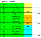
So on the sheet - You will see 9 + 2 + 7 + 18 = 36. The next one in the column is 10. This would make 46. (Column C - Pallets)
it would need to take 1 from the 10. so that 36 + 1 = 37. and then leaves the remaining 9.
So i would need the new column to show 9 2 7 18 1 9
So that stores would show up twice (Expected Outcome Image) but their start value would have been split up. Still totaling their start value though.

I had an attempt trying to use the Offset Formula and jumping back up the column but couldn't figure out how to make it consistent. Along with a lot of If statements.

Any Ideas?
 

Attachments

  • Small Sample of Data.PNG
    Small Sample of Data.PNG
    24.8 KB · Views: 18
  • Expected Outcome.PNG
    Expected Outcome.PNG
    10.7 KB · Views: 19

Excel Facts

What do {} around a formula in the formula bar mean?
{Formula} means the formula was entered using Ctrl+Shift+Enter signifying an old-style array formula.
Welcome to the MrExcel forum!

Your request requires adding extra rows when you need to split a store. This means that a traditional formula won't work, since formulas return values, they don't rearrange elements of the sheet. It's conceivable that a complex enough LAMBDA formula might work, but I don't think that will work for you, since it would require that the original data remain in place, and the revised version would have to be somewhere else.

This leaves VBA (the Excel scripting language). That is capable of calculating the values you want, as well as permanently adding new rows where needed. Is this of interest for you? If so, I can write something up. How many rows, more or less, is in your table? Do you want the results returned in the same place, or somewhere else? I notice in your picture that you have filtering on. Would you want the results based on the entire table, or if you filter by something? Do you want the highlighting as shown in your outcome picture, or was that merely for illustration?
 
Upvote 0
Welcome to the MrExcel forum!

Your request requires adding extra rows when you need to split a store. This means that a traditional formula won't work, since formulas return values, they don't rearrange elements of the sheet. It's conceivable that a complex enough LAMBDA formula might work, but I don't think that will work for you, since it would require that the original data remain in place, and the revised version would have to be somewhere else.

This leaves VBA (the Excel scripting language). That is capable of calculating the values you want, as well as permanently adding new rows where needed. Is this of interest for you? If so, I can write something up. How many rows, more or less, is in your table? Do you want the results returned in the same place, or somewhere else? I notice in your picture that you have filtering on. Would you want the results based on the entire table, or if you filter by something? Do you want the highlighting as shown in your outcome picture, or was that merely for illustration?
Hi, Yes this is of interest to me.

At one time, i would say there is no more than around 200 Rows of Data. Apologies if it looks filter because of it being in a table format. I filter the data first and then copy the remaining data onto another sheet so no need to worry about filtering the data first. I can filter it and then copy the data onto the page with the macro.

If the result of the Macro can be shown onto a different tab. that's fine with me. Doesn't need to be in the same place as the data.

I would want the results to be off the entire table. Whatever data i put into the table. Needs to be sorted

Along with the values. if you could get the other columns (store number / store name / Split along with the pallet values. That would be great.

The highlighting was just to show the difference sets that equal 37. There doesn't need to be any sort of highlighting on there but wouldn't go amiss if it was added.

I appreciate this Eric.
 
Upvote 0
OK, give this a shot.

Open a COPY of your workbook. Press Alt-F11 to open the macro editor. Press Alt-IM to insert a module. Copy the following code into the sheet that opens:

VBA Code:
Sub SplitPallets()
Dim UpperLeft As Range, Results As Range
Dim NumCols As Long, NumRows As Long, c As Long, r As Long, r2 As Long, RunningTotal As Long
Dim SplitValue As Long, PalletCol As Long
Dim output() As Variant, MyData As Variant

    Set UpperLeft = Range("A1")
    Set Results = Range("G1")
    SplitValue = 37
    PalletCol = 3
    
    NumCols = UpperLeft.End(xlToRight).Column - UpperLeft.Column + 1
    NumRows = UpperLeft.End(xlDown).Row - UpperLeft.Row
    
    ReDim output(1 To NumRows * 2, 1 To NumCols)
    MyData = UpperLeft.Offset(1).Resize(NumRows, NumCols).Value
    
    r2 = 0
    RunningTotal = 0
    
    For r = 1 To NumRows
        
        r2 = r2 + 1
        For c = 1 To NumCols
            output(r2, c) = MyData(r, c)
        Next c

        If RunningTotal + MyData(r, PalletCol) >= SplitValue Then
            output(r2, PalletCol) = SplitValue - RunningTotal
            MyData(r, PalletCol) = MyData(r, PalletCol) - output(r2, PalletCol)
            RunningTotal = 0
            If MyData(r, PalletCol) > 0 Then r = r - 1
        Else
            RunningTotal = RunningTotal + MyData(r, PalletCol)
        End If
    Next r
    
    Results.Resize(, NumCols) = UpperLeft.Resize(, NumCols).Value
    Results.Offset(1).Resize(r2, NumCols) = output
            
End Sub

Set the "Set UpperLeft = " to the upper left corner of your table, including the headers. Set the "Set Results = " to where you want to put the results. It can be the same place if you want, it will just overwrite the original table. Actually, given that it is a table, it probably should be a new location. Make sure that the "SplitValue =" and "PalletCol = " lines have the right values. (Given that this is a table, I might have been able to leverage that somehow, but this should work fine.)

Now go back to the Excel Window. Press Alt-F8 to open the macro selector. Select the SplitPallets macro and click Run.

Below is the results of my test. The A1 range shows the original table, the G1 range shows the results.

Book2
ABCDEFGHIJ
1Store NumberStore NamePalletSplitStore NumberStore NamePalletSplit
21Jersey9DTS South1Jersey9DTS South
32IOW2DTS South2IOW2DTS South
43Ashford7DTS South3Ashford7DTS South
54Maidstone18DTS South4Maidstone18DTS South
65Sittingbourne10DTS South5Sittingbourne1DTS South
76Rustington9DTS South5Sittingbourne9DTS South
87Chichester9DTS South6Rustington9DTS South
98Bournemouth24DTS South7Chichester9DTS South
109North Shields8DTS South8Bournemouth10DTS South
1110Cramlington7DTS South8Bournemouth14DTS South
1211Durham8DTS South9North Shields8DTS South
1312Oxford12DTS South10Cramlington7DTS South
1413Swindon12DTS South11Durham8DTS South
1514Crawley1DTS South12Oxford12DTS South
1615Farnborough7DTS South13Swindon12DTS South
1716Basingstoke11DTS South14Crawley1DTS South
1817Colchester12DTS South15Farnborough7DTS South
1918IPSWICH11DTS South16Basingstoke5DTS South
2019Romford19DTS South16Basingstoke6DTS South
2120Greenford17DTS South17Colchester12DTS South
2221Feltham1DTS South18IPSWICH11DTS South
2322Aylesbury7DTS South19Romford8DTS South
2423St Albans6DTS South19Romford11DTS South
2524Dunstable18DTS South20Greenford17DTS South
2621Feltham1DTS South
2722Aylesbury7DTS South
2823St Albans1DTS South
2923St Albans5DTS South
3024Dunstable18DTS South
Sheet2


Let me know how this works!
 
Upvote 1
Solution
Hi, see the linked files for a possible solution (with param and tech sheets, without VBA)...

SplitStore1.xlsx
TargetStore:37
(your Data)

SplitStore2.xlsx
TargetStore:36
(your Data)

SplitStore3.xlsx
TargetStore:36
(modified Data)

The formulas used in the table...
tech!A2: =LET(x,INDEX(Data!A:A,ROW()),IF(x="","",x)) (Range: A2:A300 ...)
tech!B2: =LET(x,INDEX(Data!A:A,ROW()),IF(x="","",INDEX(Data!B:B,ROW()))) (Range: B2:B300 ...)
tech!C2: =LET(x,INDEX(Data!A:A,ROW()),IF(x="","",INDEX(Data!C:C,ROW()))) (Range: C2:C300 ...)
tech!D2: =LET(x,INDEX(Data!A:A,ROW()),IF(x="","",INDEX(Data!D:D,ROW()))) (Range: D2:D300 ...)
tech!E2: =IF(A2="","",SUM(C$2:C2)) (Range: E2:E300 ...)
tech!F1=1
tech!F2: =IF(A2="","",INT((E2-1)/param!B$1)+1) (Range: F2:F300 ...)
tech!G2: =IF(A2="","",F2-F1) (Range: G2:G300 ...)
tech!H2: =IF(A2="","",G2+IF(I1=0,0,1)) (Range: H2:H300 ...)
tech!I1=1
tech!I2: =IF(A2="","",MOD(E2,param!B$1)) (Range: I2:I300 ...)
tech!J1=0
tech!J2: =IF(A2="","",SUM(H$2:H2)+1) (Range: J2:J300 ...)
tech!K1=0
tech!K2: =IF(A2="","",IF(I1=0,1,L1+1)) (Range: K2:K300 ...)
tech!L1=0
tech!L2: =IF(A2="","",IF(H2=1,K2,1)) (Range: L2:L300 ...)
tech!L2: =COUNT(C:C)+SUM(G:G)-1

Outcome!A2: =IF(ROW()>tech!M$2,"",INDEX(tech!A:A,IFERROR(MATCH(ROW(),tech!J:J,0),MATCH(ROW(),tech!J:J,1)+1))) (Range: A2:A500 ...)
Outcome!B2: =IF(ROW()>tech!M$2,"",INDEX(tech!B:B,IFERROR(MATCH(ROW(),tech!J:J,0),MATCH(ROW(),tech!J:J,1)+1))) (Range: B2:B500 ...)
Outcome!C2: =LET(x,IFERROR(MATCH(ROW(),tech!J:J,0),MATCH(ROW(),tech!J:J,1)+1),y,IFERROR(MATCH(ROW(),tech!J:J,0),MATCH(ROW(),tech!J:J,1)),fx,INDEX(tech!F:F,x),jx,INDEX(tech!J:J,x),kx,INDEX(tech!K:K,x),IF(ROW()>tech!M$2,"",IF(INDEX(tech!G:G,x)=0,fx&"/"&kx,fx-jx+ROW()&"/"&IF(ROW()-INDEX(tech!J:J,y)=1,kx,"1")))) (Range: C2:C500 ...)
Outcome!D2: =LET(x,IFERROR(MATCH(ROW(),tech!J:J,0),MATCH(ROW(),tech!J:J,1)+1),y,IFERROR(MATCH(ROW(),tech!J:J,0),MATCH(ROW(),tech!J:J,1)),cx,INDEX(tech!C:C,x),ix,INDEX(tech!I:I,x),IF(ROW()>tech!M$2,"",IF(INDEX(tech!G:G,x)=0,cx,IF(ROW()-INDEX(tech!J:J,y)=1,MIN(cx,param!B$1-INDEX(tech!I:I,y)),IF(OR(ROW()<INDEX(tech!J:J,x),ix=0),param!B$1,ix))))) (Range: D2:D500 ...)

The formulas for Conditional Formatting
=AND(D1>0,MOD(IFERROR(VALUE(LEFT(C1,SEARCH("/",C1)-1)),0),3)=1)
=AND(D1>0,MOD(IFERROR(VALUE(LEFT(C1,SEARCH("/",C1)-1)),0),3)=2)
=AND(D1>0,MOD(IFERROR(VALUE(LEFT(C1,SEARCH("/",C1)-1)),0),3)=0)

SplitStore1.xlsx
SplitStore2.xlsx
SplitStore3.xlsx

SplitStore1Data.png


SplitStore1param.png


SplitStore1tech.png


SplitStore1Outcome.png


SplitStore3Data.png


SplitStore3param.png


SplitStore3tech.png


SplitStore3Outcome.png
 
Upvote 0
OK, give this a shot.

Open a COPY of your workbook. Press Alt-F11 to open the macro editor. Press Alt-IM to insert a module. Copy the following code into the sheet that opens:

VBA Code:
Sub SplitPallets()
Dim UpperLeft As Range, Results As Range
Dim NumCols As Long, NumRows As Long, c As Long, r As Long, r2 As Long, RunningTotal As Long
Dim SplitValue As Long, PalletCol As Long
Dim output() As Variant, MyData As Variant

    Set UpperLeft = Range("A1")
    Set Results = Range("G1")
    SplitValue = 37
    PalletCol = 3
  
    NumCols = UpperLeft.End(xlToRight).Column - UpperLeft.Column + 1
    NumRows = UpperLeft.End(xlDown).Row - UpperLeft.Row
  
    ReDim output(1 To NumRows * 2, 1 To NumCols)
    MyData = UpperLeft.Offset(1).Resize(NumRows, NumCols).Value
  
    r2 = 0
    RunningTotal = 0
  
    For r = 1 To NumRows
      
        r2 = r2 + 1
        For c = 1 To NumCols
            output(r2, c) = MyData(r, c)
        Next c

        If RunningTotal + MyData(r, PalletCol) >= SplitValue Then
            output(r2, PalletCol) = SplitValue - RunningTotal
            MyData(r, PalletCol) = MyData(r, PalletCol) - output(r2, PalletCol)
            RunningTotal = 0
            If MyData(r, PalletCol) > 0 Then r = r - 1
        Else
            RunningTotal = RunningTotal + MyData(r, PalletCol)
        End If
    Next r
  
    Results.Resize(, NumCols) = UpperLeft.Resize(, NumCols).Value
    Results.Offset(1).Resize(r2, NumCols) = output
          
End Sub

Set the "Set UpperLeft = " to the upper left corner of your table, including the headers. Set the "Set Results = " to where you want to put the results. It can be the same place if you want, it will just overwrite the original table. Actually, given that it is a table, it probably should be a new location. Make sure that the "SplitValue =" and "PalletCol = " lines have the right values. (Given that this is a table, I might have been able to leverage that somehow, but this should work fine.)

Now go back to the Excel Window. Press Alt-F8 to open the macro selector. Select the SplitPallets macro and click Run.

Below is the results of my test. The A1 range shows the original table, the G1 range shows the results.

Book2
ABCDEFGHIJ
1Store NumberStore NamePalletSplitStore NumberStore NamePalletSplit
21Jersey9DTS South1Jersey9DTS South
32IOW2DTS South2IOW2DTS South
43Ashford7DTS South3Ashford7DTS South
54Maidstone18DTS South4Maidstone18DTS South
65Sittingbourne10DTS South5Sittingbourne1DTS South
76Rustington9DTS South5Sittingbourne9DTS South
87Chichester9DTS South6Rustington9DTS South
98Bournemouth24DTS South7Chichester9DTS South
109North Shields8DTS South8Bournemouth10DTS South
1110Cramlington7DTS South8Bournemouth14DTS South
1211Durham8DTS South9North Shields8DTS South
1312Oxford12DTS South10Cramlington7DTS South
1413Swindon12DTS South11Durham8DTS South
1514Crawley1DTS South12Oxford12DTS South
1615Farnborough7DTS South13Swindon12DTS South
1716Basingstoke11DTS South14Crawley1DTS South
1817Colchester12DTS South15Farnborough7DTS South
1918IPSWICH11DTS South16Basingstoke5DTS South
2019Romford19DTS South16Basingstoke6DTS South
2120Greenford17DTS South17Colchester12DTS South
2221Feltham1DTS South18IPSWICH11DTS South
2322Aylesbury7DTS South19Romford8DTS South
2423St Albans6DTS South19Romford11DTS South
2524Dunstable18DTS South20Greenford17DTS South
2621Feltham1DTS South
2722Aylesbury7DTS South
2823St Albans1DTS South
2923St Albans5DTS South
3024Dunstable18DTS South
Sheet2


Let me know how this works!
Hi Eric,

Just tested the VBA out and it works beautifully.

Thank you so much for figuring this out.

I might be checky for asking this but if i wanted to add a new row everytime the pallet total hit 37. The new row would say

How would i go about doing this?

So it would work the same way - just includes a new row to seperate all the sections that = 37
 
Upvote 0
Adding a new row is easy enough. Look for this line:

VBA Code:
If MyData(r, PalletCol) > 0 Then r = r - 1


and add a line after it like this:

VBA Code:
If MyData(r, PalletCol) > 0 Then r = r - 1
r2 = r2 + 1


If you want that line to say something in particular:

VBA Code:
If MyData(r, PalletCol) > 0 Then r = r - 1
r2 = r2 + 1
output(r2, PalletCol) = "----------"


You can change the PalletCol to any column number if you want the text somewhere else.
 
Upvote 0
HI Eric,

That perfect, I was able to edit it to show what I wanted in the new row.

Only Issue im having is its not inserting the text into the last row (this one is the one that doesn't get over 37 pallets so I'm assuming this is the issue.

So all the other inserted rows are fine. Just the final one and i can't find where in the code to edit it to allow me to insert text like the other rows.
 
Upvote 0
After the

VBA Code:
Next r


line, put

VBA Code:
Next r

If RunningTotal > 0 Then
    r2 = r2 + 1
    output(r2, PalletCol) = "your text"
End If


using your text of course.
 
Upvote 0

Forum statistics

Threads
1,214,591
Messages
6,120,427
Members
448,961
Latest member
nzskater

We've detected that you are using an adblocker.

We have a great community of people providing Excel help here, but the hosting costs are enormous. You can help keep this site running by allowing ads on MrExcel.com.
Allow Ads at MrExcel

Which adblocker are you using?

Disable AdBlock

Follow these easy steps to disable AdBlock

1)Click on the icon in the browser’s toolbar.
2)Click on the icon in the browser’s toolbar.
2)Click on the "Pause on this site" option.
Go back

Disable AdBlock Plus

Follow these easy steps to disable AdBlock Plus

1)Click on the icon in the browser’s toolbar.
2)Click on the toggle to disable it for "mrexcel.com".
Go back

Disable uBlock Origin

Follow these easy steps to disable uBlock Origin

1)Click on the icon in the browser’s toolbar.
2)Click on the "Power" button.
3)Click on the "Refresh" button.
Go back

Disable uBlock

Follow these easy steps to disable uBlock

1)Click on the icon in the browser’s toolbar.
2)Click on the "Power" button.
3)Click on the "Refresh" button.
Go back
Back
Top