Vincent88
Active Member
- Joined
- Mar 5, 2021
- Messages
- 382
- Office Version
- 2019
- Platform
- Windows
- Mobile
Hi Guy, need help to modify the code to add one more condition to trigger the change.
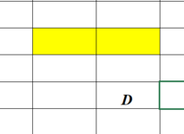
If the 1st cell value is "N' and adjacent cell value is "E", then change border style of both cells.
Also how to add code to let the change restore to original (no change) when conditions not met.
Thanks
If the 1st cell value is "N' and adjacent cell value is "E", then change border style of both cells.
Also how to add code to let the change restore to original (no change) when conditions not met.
Thanks
VBA Code:
Dim c As Range, rng As Range, rng1 As Range
Set rng = Range("C3", Range("AL" & Rows.Count).End(xlUp))
For Each c In rng
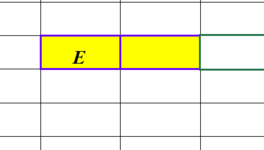
Select Case UCase(c.Value)
Case "E", "N"
Select Case UCase(c.Offset(, 1).Value)
Case "D", "G"
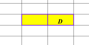
Set rng1 = c.Resize(1, 2)
With rng1
.Borders.LineStyle = xlContinuous
.Borders.Weight = xlThick
'.Borders.Color = vbBlue
.Borders.Color = RGB(102, 0, 255)
End With
End Select
End Select
Next
End If
End If
End Sub