Advanced Rows Combine

[Katterman]

Hello All

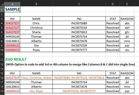
I'm looking for some assistance in creating a macro that will finds duplicate rows based on a specific cell, combine one or two other cell's values in that row (separating values by a comma space or just space) and leaving just the one row. This example shows just 1 column of combined values but more may be needed, but still based of the primary Duplicate value.

Original	End Result

<tbody>
</tbody>

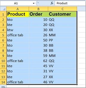
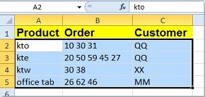
I have found some Similar VBA code HERE but the code itself only works for 2 columns.
Further down below the code and under This Category (Combine multiple duplicate rows into one Kutools for Excel)
is exactly what i'm looking for in a macro only (No Excel Interfaces required). More Info also HERE

Note: I do have a Legally Licensed copy of this KuTools Add In (And Love it) but i need a macro
for a project that multiple users will be needing this function for and obtaining multiple user licenses are not an option due to the costs attributed..
I also am unable to pull out a macro used in this add-on since it's locked down, for Obvious and respected proprietary reasons.

Thanks Everyone in Advance for Reading and possibly assisting.

Scott

 

[Katterman]

Anyone able to assist here?

Many Thanks Again in Advance.

Scott

 

[rakeshp2010]

I am trying to understand the output here. kto has three values i.e. 10,30, 31 for different customers. However, the customer you have entered in smaller table is just one - QQ?!

 

[Katterman]

Hello. Thanks for your reply.

In my example with the final image, the company column was not chosen as a second field to be merged. Only the one column was chosen with the number values. Although, my initial request is to have the option built into the macro to allow additional columns to merge data as you point out in this reply.

Hope that made sense and thanks for looking at this.

Scott

 

[bhos123]

https://www.mrexcel.com/forum/excel-questions/953739-merging-duplicate-fields.html

 

[Katterman]

https://www.mrexcel.com/forum/excel-questions/953739-merging-duplicate-fields.html

Hello bhos123

Thanks so much for your reply.
I looked at the link you sent and with a small tweak, that works the way i need in general.
I basically removed the

[COLOR=#333333]And Cells(i, 2).Value = Cells(i - 1, 2).Value [/COLOR]

as i only need one column to be checked for Duplicates and merged and it works as needed.

One additional option i need, and not having any luck tweaking your code to make work,
is to have a second or 3rd column added (maybe a couple more) that will also merge the data
into a single row the same way. End result would be the same except more cells would contained
merged data separated by a comma.

Thanks Again for your help

Scott

 

[bhos123]

you want to put conditions on more than 2 columns?? or you want to merge the data in more than 2 rows for matching in a single column.?

 

[Katterman]

you want to put conditions on more than 2 columns?? or you want to merge the data in more than 2 rows for matching in a single column.?

Hello
The end Goal is to find all duplicate rows based on the values in Column A (for example) and then merge values of one or more other columns.

Here's a sample image:

Your code works great for my needs once i removed that piece i noted previously as i'm not validating 2 columns for Duplicates. Just one.
The only thing I'm requesting is to be able to merge 2 or more columns as in the example image. Data in the non merged cells does not matter in regards to which on the duplicate rows is kept .

Hope that helps and thanks again for your time and efforts

Scott

 

[bhos123]

Sub macro1()
Dim lngLastRow As String
Dim lastRow As Long
Dim lastcolumn As Long
Application.ScreenUpdating = False


lastRow = ActiveSheet.UsedRange.Row - 1 + ActiveSheet.UsedRange.Rows.Count
lastcolumn = ActiveSheet.UsedRange.Column - 1 + ActiveSheet.UsedRange.Columns.Count


ActiveSheet.Sort.SortFields.Clear
ActiveSheet.Sort.SortFields.Add Key:=Range(Cells(2, 1), Cells(lastRow, 1)), _
SortOn:=xlSortOnValues, Order:=xlAscending, DataOption:=xlSortNormal


With ActiveSheet.Sort
.SetRange Range(Cells(1, 1), Cells(lastRow, lastcolumn))
.Header = xlYes
.MatchCase = False
.Orientation = xlTopToBottom
.SortMethod = xlPinYin
.Apply
End With


For i = lastRow To 2 Step -1


If Cells(i, 1).Value = Cells(i - 1, 1).Value Then
Cells(i - 1, 2).Value = Cells(i - 1, 2).Value & " , " & Cells(i, 2).Value
Cells(i - 1, 3).Value = Cells(i - 1, 3).Value & " , " & Cells(i, 3).Value


Rows(i).EntireRow.Delete
End If


Next
Application.ScreenUpdating = True


End Sub

 

[Katterman]

THANKS So Much bhos123.

This works Perfectly and exactly what i needed.
And also easy to add more merging columns if needed.

Again, Thanks so much for your time and efforts here.

Scott