Hi! So I'll give some background so what I am trying to achieve makes sense.
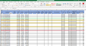
The screenshot is of me, assessing photos of roads for flood damage.
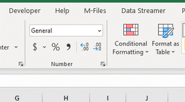
Where the damage starts, I highlight the row and hit "GOOD" up in the styles format (on the top ribbon).
When I have photos that show evidence of the damage I highlight the row and hit "NEUTRAL" up in the styles format.
When the treatment ends, again I highlight that row and hit "BAD" in the styles format.
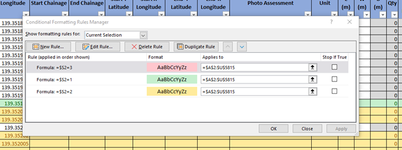
I use these colors because the "regular" yellow red and green are glaringly bright and when we assess damage for months at a time, it can really hurt the eyes.
Row S wasn't always there, it is there for me trying to spitball ideas and make the above process more efficient. The actual choosing of the colors isn't so bad, is the having to highlight the whole row.
I work with two computer screens so I have the workbook on one screen and the photos on the other screen.
As you can see, the row is selected from A to U (normally T but I added S today)
What is something I can do that will select the range of cells easily OR color them for me with a number or other data in the S column? it would be awesome to be able to just use the number pad and hit numbers that color the lines in the range or any other shortcut someone can think of?
The more efficient I can make this process, the more roads we can assess and the faster the community gets safer roads to drive on. Sometimes these assessments are needed ASAP.
The screenshot is of me, assessing photos of roads for flood damage.
Where the damage starts, I highlight the row and hit "GOOD" up in the styles format (on the top ribbon).
When I have photos that show evidence of the damage I highlight the row and hit "NEUTRAL" up in the styles format.
When the treatment ends, again I highlight that row and hit "BAD" in the styles format.
I use these colors because the "regular" yellow red and green are glaringly bright and when we assess damage for months at a time, it can really hurt the eyes.
Row S wasn't always there, it is there for me trying to spitball ideas and make the above process more efficient. The actual choosing of the colors isn't so bad, is the having to highlight the whole row.
I work with two computer screens so I have the workbook on one screen and the photos on the other screen.
As you can see, the row is selected from A to U (normally T but I added S today)
What is something I can do that will select the range of cells easily OR color them for me with a number or other data in the S column? it would be awesome to be able to just use the number pad and hit numbers that color the lines in the range or any other shortcut someone can think of?
The more efficient I can make this process, the more roads we can assess and the faster the community gets safer roads to drive on. Sometimes these assessments are needed ASAP.
")