Hello,
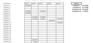
I have a spreadsheet of Assets across C:CA and in Col B I have a list of companies that could own those assets. Many of the same companies own multiple assets in varying percentages. As you can see from the simplified example photo, there are lots of blank spaces and there is a litter of percentage numbers. Of course if you sum the percentages in any column, the total will always equal 100%.
I would like to use another tab to go into the Ownership tab and ignore the blank spaces so that when I select an asset on a dropdown or similar, when Asset 1 comes up, then the formula will go and grab the equity positions and fill them in the cells under the name ignoring all the blank spaces. It will never be the case that an asset will have more than 7 owners and I am fine with blank cells if there is less than 7 owners.
I am using Index/Aggregate where I am searching for any value above basically zero and dividing that by itself to tease out the TRUE references, but I am unable to find a way to do this dynamically - as you can see in the formula below, this is only searching Col C for Asset 1 and when I want to find the ownership in Asset 2 (for example, I am copy and pasting the formula and then doing a Find/Replace for the col ref).
Is there a simple way to search for the column heading e.g. Asset 2, then apply the relevant INDEX/AGGREGATE below without VBA? I have tried to use INDEX/MATCH but I don't think the syntax works.
I have attached a simplified example of the data set and the cluster in Bold on the right would be the end result and imagine that the heading in bold (Asset 2) could be dropped down to any asset name and the data would refresh underneath ignoring all the empty rows that are in the relevant columns.
=INDEX('Ownership'!$C$6:$C$60,AGGREGATE(15,3,(IF('Ownership'!$C$6:$C$60>0.001,TRUE,FALSE)/IF('Ownership'!$C$6:$C$60>0.001,TRUE,FALSE))*(ROW('Ownership'!$C$6:$C$60)-ROW('Ownership'!$C$5)),ROWS($A$1:A1)))
Apologies if this is an obvious one to solve but I am struggling to adjust the above formula to solve the issue.
P.S. Even more desirable would be if they were called into the simplified list in order of highest to lowest equity position and if there was a way to tag the managing owner of the Asset (which will always only be one company), which may not be the company with the biggest equity position. I was thinking that in my data entry I could mark the percentage interest of the managing partner in Green and if the formula could find a way to pull that in and maybe concatenate the Company name to for example "Company 1 Managing Owner" or tag it in some way (even just make it bold) But I don't know if that is possible.
Thanks,
S