Applying Conditional Formatting without overwriting existing formatting

[TGreenwood]

Good morning

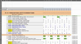
I am trying to set up conditional formatting on a spreadsheet. I've it set up correctly on the top row, and wish to apply it to the rest of the sheet.
However, I don't want to simply drag it down as it overwrites the existing formatting (not conditional).
Is there any way I can get the Conditional Formatting to apply to the rest of the sheet using a method other than the standard copy/paste/Format Painter etc?

Format Rule:
=$D13='Audit Exam task'!$H$3:$H$5

Applies to:
=$A$13:$S$13

I need it to cover every row on the sheet. I am aware that if the formula is true, it will overwrite the formatting, which I am fine with.

Thank you

 

[RoryA]

Welcome to the forum.

Just edit the 13 at the end of the Applies To range to whatever row number you need. Note that unless H3:H5 is a merged cell, your current formula doesn't really make sense.

 

[TGreenwood]

Welcome to the forum.

Just edit the 13 at the end of the Applies To range to whatever row number you need. Note that unless H3:H5 is a merged cell, your current formula doesn't really make sense.

Thanks Rory, but that hasn't worked?

And yes, H3:H5 is a merged cell.

 

[RoryA]

What exactly does "hasn't worked" mean? I do this frequently, so I know it works.

 

[TGreenwood]

What exactly does "hasn't worked" mean? I do this frequently, so I know it works.

I updated the Applied To range, and tested it, but the top line stayed green, not the one I was testing.

 

[TGreenwood]

What exactly does "hasn't worked" mean? I do this frequently, so I know it works.

Do I need to change the cell ref in the formula?

 

[RoryA]

No, since you used a relative row number in the $D13 part. (I'm assuming that you need to compare all rows to H3)

Did you change the value in D13 as well? If not, I'd expect it to remain green.

 

[TGreenwood]

No, since you used a relative row number in the $D13 part. (I'm assuming that you need to compare all rows to H3)

Did you change the value in D13 as well? If not, I'd expect it to remain green.

No, I changed the value in H3:H5, and want the corresponding row to highlight green, not D13.
e.g.: If the value in D34 is in H3:H5, then row 34 will highlight.

 

[RoryA]

So what do your Formula and Applies To boxes look like now?

 

[TGreenwood]

Format Rule:
=$D13='Audit Exam task'!$H$3:$H$5

Applies to:
=$A$13:$S$34