Applying intuitive formatting to a spreadsheet of client data

[Legion_1984]

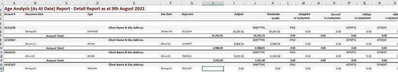
I have a spreadsheet with 14,500 lines of data, I was able to apply VBA codes to remove blank rows and columns to get it down to 8,000 but I need to apply formatting to the rows (column A if it contains an account # to shade fill the whole row in the selection) and applying a top and thick bottom border to any row with "Account Total" in Column C

Capture of a sample of the data attached - this is how I would like to carry the formatting through the entire selection area - any help / guidance would be a huge help! Thanks in advance.

 

[Peter_SSs]

Welcome to the MrExcel board!

Typically you would use Excel's built-in Conditional Formatting for that sort of job since it automatically adjusts if the data changes. However, CF does not cater for thick borders.

In any case you may have been specifically looking for more vba to add to your existing code. You could give this a try with a copy of your workbook

Sub ApplyFormatting()
  Application.ScreenUpdating = False
  With Intersect(ActiveSheet.UsedRange, Rows("4:" & Range("C" & Rows.Count).End(xlUp).Row))
    .AutoFilter Field:=1, Criteria1:="<>"
    .Offset(1).Resize(.Rows.Count - 1).Interior.Color = 14277081
    .AutoFilter Field:=1
    .AutoFilter Field:=3, Criteria1:="Account Total"
    With .Offset(1).Resize(.Rows.Count - 1)
      .Borders(xlEdgeTop).LineStyle = xlContinuous
      .Borders(xlEdgeBottom).LineStyle = xlContinuous
      .Borders(xlEdgeBottom).Weight = xlThick
    End With
    .Parent.AutoFilterMode = False
  End With
  Application.ScreenUpdating = True
End Sub

 

[Legion_1984]

Sub ApplyFormatting() Application.ScreenUpdating = False With Intersect(ActiveSheet.UsedRange, Rows("4:" & Range("C" & Rows.Count).End(xlUp).Row)) .AutoFilter Field:=1, Criteria1:="<>" .Offset(1).Resize(.Rows.Count - 1).Interior.Color = 14277081 .AutoFilter Field:=1 .AutoFilter Field:=3, Criteria1:="Account Total" With .Offset(1).Resize(.Rows.Count - 1) .Borders(xlEdgeTop).LineStyle = xlContinuous .Borders(xlEdgeBottom).LineStyle = xlContinuous .Borders(xlEdgeBottom).Weight = xlThick End With .Parent.AutoFilterMode = False End With Application.ScreenUpdating = True End Sub

THANK YOU! I tried the conditional formatting for the shading but I think my formula logic was off - it would apply to the line above or below the account # fields holding data, then I considered that combining them in VBA might simplify the editing.
Seriously thank you - this has saved hours!

 

[Peter_SSs]

You're welcome. Thanks for the follow-up.