Arrange the numbers as per box range

[motilulla]

Hello,

I need help to arrange 8 random number min = 1 max = 24 in the 6 boxes each box is filled with 4 numbers

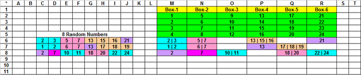
For example in the cells C6:J6 I got 8 random numbers in ascending order i need to put them under each box with their corresponding value 2 & 3 go in the cell = M6, 5 & 7 go in the cell = N6, 13, 15 & 16 go in the cell = P6, 21 go in the cell = R6

With the same way row 7.... 8 & so on

For more detail the image is attached.

*	A	B	C	D	E	F	G	H	I	J	K	L	M	N	O	P	Q	R	S	T
1													Box-1	Box-2	Box-3	Box-4	Box-5	Box-6
2													1	5	9	13	17	21
3													2	6	10	14	18	22
4													3	7	11	15	19	23
5													4	8	12	16	20	24
6			2	3	5	7	13	15	16	21			2 | 3	5 | 7		13 | 15 | 16		21
7			1	2	6	7	13	17	18	19			1 | 2	6 | 7		13	17 | 18 | 19
8			2	7	10	11	18	20	22	24			2	7	10 | 11		18 | 20	22 | 24
9
10
11

Thank you all.

I am using Excel 2000

Regards,
Moti

 

[jasonb75]

See if this works. I doubt that many people on here (if any) will be able to test in excel 2000 so it will likely involve an amount of trial and error.
Note that you will need to add the vba code before entering the formula.

Function aconcat(a As Variant, Optional sep As String = "") As String
    ' Harlan Grove, Mar 2002
    ' With a minor edit to ignore blanks
Dim y As Variant
If TypeOf a Is Range Then
    For Each y In a.Cells
        If Len(y.Value) > 0 Then aconcat = aconcat & y.Value & sep
    Next y
ElseIf IsArray(a) Then
    For Each y In a
        If Len(y) > 0 Then aconcat = aconcat & y & sep
    Next y
Else
    aconcat = aconcat & a & sep
End If
    If Len(aconcat) > 0 Then aconcat = Left(aconcat, Len(aconcat) - Len(sep)) Else aconcat = ""
End Function

Book1
	C	D	E	F	G	H	I	J	K	L	M	N	O	P	Q	R
1											Box-1	Box-2	Box-3	Box-4	Box-5	Box-6
2											1	5	9	13	17	21
3											2	6	10	14	18	22
4											3	7	11	15	19	23
5											4	8	12	16	20	24
6	2	3	5	7	13	15	16	21			2 | 3	5 | 7		13 | 15 | 16		21
7	1	2	6	7	13	17	18	19			1 | 2	6 | 7		13	17 | 18 | 19
8	2	7	10	11	18	20	22	24			2	7	10 | 11		18 | 20	22 | 24
Sheet2

Cell Formulas
Range	Formula
M6:R8	M6	=aconcat(IFERROR(IF(LOOKUP($C6:$J6,M$2:M$5)=$C6:$J6,$C6:$J6,""),"")," | ")
Press CTRL+SHIFT+ENTER to enter array formulas.

 

[motilulla]

See if this works. I doubt that many people on here (if any) will be able to test in excel 2000 so it will likely involve an amount of trial and error.
Note that you will need to add the vba code before entering the formula.
22 | 24[/XD][/XR][/RANGE]

Cell Formulas
Range	Formula
M6:R8	M6	=aconcat(IFERROR(IF(LOOKUP($C6:$J6,M$2:M$5)=$C6:$J6,$C6:$J6,""),"")," | ")
Press CTRL+SHIFT+ENTER to enter array formulas.

jasonb75, I install the function as per your instruction after i applied a formula got a #VALUE! error, it is because "IFERROR" function does not work in Excel 2000.

I appreciate your help and time you took to make a function.

One question instead function it can't be made macro?

Kind Regards,
Moti

 

[Marc L]

Hello, a VBA demonstration for starters :​

Sub Demo1()
          Dim W, C%, V(), R&, X, Y
    With [M1].CurrentRegion.Rows("2:5").Columns
        ReDim W(1 To .Count)
        For C = 1 To .Count:  W(C) = Application.Transpose(.Item(C)):  Next
    End With
    With [C6].CurrentRegion.Rows
        ReDim V(1 To .Count, 1 To UBound(W))
        For R = 1 To .Count
            X = Application.Index(.Item(R).Value2, 1, 0)
        For C = 1 To UBound(W)
            Y = Filter(Application.IfError(Application.Match(W(C), X, 0), False), False, False)
            If UBound(Y) > -1 Then V(R, C) = Join(Application.Index(X, 1, Y), "|")
        Next C, R
            [M6].Resize(.Count, UBound(W)).Value2 = V
    End With
End Sub

 

[motilulla]

Hello, a VBA demonstration for starters :​

Sub Demo1()
          Dim W, C%, V(), R&, X, Y
    With [M1].CurrentRegion.Rows("2:5").Columns
        ReDim W(1 To .Count)
        For C = 1 To .Count:  W(C) = Application.Transpose(.Item(C)):  Next
    End With
    With [C6].CurrentRegion.Rows
        ReDim V(1 To .Count, 1 To UBound(W))
        For R = 1 To .Count
            X = Application.Index(.Item(R).Value2, 1, 0)
        For C = 1 To UBound(W)
            Y = Filter(Application.IfError(Application.Match(W(C), X, 0), False), False, False)
            If UBound(Y) > -1 Then V(R, C) = Join(Application.Index(X, 1, Y), "|")
        Next C, R
            [M6].Resize(.Count, UBound(W)).Value2 = V
    End With
End Sub

Marc L, After running a macro I get highlighted the line below in colour yellow wit error '438'

Please can you take a look?

I appreciate your help and time you took to build a macro.

Y = Filter(Application.IfError(Application.Match(W(C), X, 0), False), False, False)

Kind Regards,
Moti

 

[Marc L]

My demonstration revamped for Excel versions prior to 2007 version :​

Sub Demo1()
          Dim W, C%, V(), R&, X, Y, K%
    With [M1].CurrentRegion.Rows("2:5").Columns
        ReDim W(1 To .Count)
        For C = 1 To .Count:  W(C) = Application.Transpose(.Item(C)):  Next
    End With
    With [C6].CurrentRegion.Rows
        ReDim V(1 To .Count, 1 To UBound(W))
        For R = 1 To .Count
            X = Application.Index(.Item(R).Value2, 1, 0)
        For C = 1 To UBound(W)
            Y = Application.Match(W(C), X, 0)
        For K = 1 To UBound(Y)
            If IsError(Y(K)) Then Y(K) = False
        Next K
            Y = Filter(Y, False, False)
            If UBound(Y) > -1 Then V(R, C) = Join(Application.Index(X, 1, Y), "|")
        Next C, R
            [M6].Resize(.Count, UBound(W)).Value2 = V
    End With
End Sub

 

[Marc L]

A little optimization :​

Sub Demo1r()
          Dim W, C%, V(), R&, X, K%
    With [M1].CurrentRegion.Rows("2:5").Columns
        ReDim W(1 To .Count)
        For C = 1 To .Count:  W(C) = Application.Transpose(.Item(C)):  Next
    End With
    With [C6].CurrentRegion.Rows
        ReDim V(1 To .Count, 1 To UBound(W))
        For R = 1 To .Count
        For C = 1 To UBound(W)
            X = Application.Match(W(C), .Item(R), 0)
        For K = 1 To UBound(X)
            If IsError(X(K)) Then X(K) = False
        Next K
            X = Filter(X, False, False)
            If UBound(X) > -1 Then V(R, C) = Join(Application.Index(.Item(R), 1, X), "|")
        Next C, R
            [M6].Resize(.Count, UBound(W)).Value2 = V
    End With
End Sub

 

[motilulla]

My demonstration revamped for Excel versions prior to 2007 version :​

Sub Demo1()
          Dim W, C%, V(), R&, X, Y, K%
    With [M1].CurrentRegion.Rows("2:5").Columns
        ReDim W(1 To .Count)
        For C = 1 To .Count:  W(C) = Application.Transpose(.Item(C)):  Next
    End With
    With [C6].CurrentRegion.Rows
        ReDim V(1 To .Count, 1 To UBound(W))
        For R = 1 To .Count
            X = Application.Index(.Item(R).Value2, 1, 0)
        For C = 1 To UBound(W)
            Y = Application.Match(W(C), X, 0)
        For K = 1 To UBound(Y)
            If IsError(Y(K)) Then Y(K) = False
        Next K
            Y = Filter(Y, False, False)
            If UBound(Y) > -1 Then V(R, C) = Join(Application.Index(X, 1, Y), "|")
        Next C, R
            [M6].Resize(.Count, UBound(W)).Value2 = V
    End With
End Sub

Marc L, Yes this worked fine only it is placing result starting from M7 instead of M6 i played a bit with the line below but cannot get it sort out. Could you tell me how can which line has to be altered?

I appreciate your help and time you took to build a macro.

[M6].Resize(.Count, UBound(W)).Value2 = V

Good Luck have a nice weekend.

Kind Regards,
Moti

 

[Marc L]

​

As obviously this codeline places the result to cell M6 so it means there is no match in C6:J6 …​

 

[motilulla]

​

As obviously this codeline places the result to cell M6 so it means there is no match in C6:J6 …​

Marc L, Please see the image attached why i am getting result starting from M7 ?