Assigning Rank to Text and Creating Colour Scaling Accordingly

[Smok3y]

Hi there,

I'm looking for a way to colour scale a table that contains text, based on rankings assigned to that text (essentially pairing ordinal ranks with nominal data, and carrying those ranks across as a means to provide colour scaling).

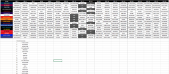
Example image attached - basically I want the table cells that contain higher ranked nominal data (in this case team names in the power rankings) to appear red and scale down from there (shades of red, orange, yellow and green).

Ideally this would entail a customisable solution, where the power rankings can change and table colour scaling updates accordingly from there.

Any help would be greatly appreciated

Cheers, Smok3y.

 

[aRandomHelper]

Possible, but you would have to create a rule for each rank. Something like this:

Book1.xlsm
	L	M	N	O	P	Q	R	S	T
1						xyz	ghi	abc	abc
2	1	abc				def	def		def
3	2	def				ghi	abc		xyz
4	3	ghi				jkl	jkl	def	jkl
5	4	jkl				xyz		xyz
6	5	xyz
Sheet7

Cells with Conditional Formatting
Cell	Condition		Cell Format	Stop If True
Q1:T5	Expression	=INDEX($L:$L,MATCH(Q1,$M:$M,0))=3	text	NO
Q1:T5	Expression	=INDEX($L:$L,MATCH(Q1,$M:$M,0))=2	text	NO
Q1:T5	Expression	=INDEX($L:$L,MATCH(Q1,$M:$M,0))=1	text	NO

 

[Smok3y]

Possible, but you would have to create a rule for each rank. Something like this:

Book1.xlsm
	L	M	N	O	P	Q	R	S	T
1						xyz	ghi	abc	abc
2	1	abc				def	def		def
3	2	def				ghi	abc		xyz
4	3	ghi				jkl	jkl	def	jkl
5	4	jkl				xyz		xyz
6	5	xyz
Sheet7

Cells with Conditional Formatting
Cell	Condition		Cell Format	Stop If True
Q1:T5	Expression	=INDEX($L:$L,MATCH(Q1,$M:$M,0))=3	text	NO
Q1:T5	Expression	=INDEX($L:$L,MATCH(Q1,$M:$M,0))=2	text	NO
Q1:T5	Expression	=INDEX($L:$L,MATCH(Q1,$M:$M,0))=1	text	NO

Thanks so much for the reply.

I'm having trouble translating your example across to mine, not sure where I am going wrong.

Would this be in Conditional Formatting? What is the Stop If True column? Bit confused how this works if only the first table cell (Q1) is referenced in the formula.

Can you step this out if possible? Apologies I haven't come across one like this before.

Cheers, Smok3y.

 

[aRandomHelper]

Would this be in Conditional Formatting? What is the Stop If True column?

Yes, that's in conditional formatting. Stop If True is a checkbox column available when you look at "Manage rules". If checked, Excel will stop at the matching condition and will not keep looking at the conditions down the list for another match. Most of the time this is not necessary, unless you have possible overlapping conditions to check.

Bit confused how this works if only the first table cell (Q1) is referenced in the formula.

The referenced cell is relative (Q1), and not absolute ($Q$1), so the referenced relative cell is actually "moving" as you apply it to a range of cells.
If you reference A1 in a range of A1:B2 the referenced cell moves as Excel looks at B1, A2, B2, etc. Some examples of how the cell is being "changed" to for each type of referencing.
A1:
A1|B1
A2|B2

$A1:
A1|A1
A2|A2

A$1:
A1|B1
A1|B1

$A$1:
A1|A1
A1|A1

I'm having trouble translating your example across to mine, not sure where I am going wrong.

So to apply the formula to your sheet, you need to break down the formula first.
These are the 3 components to change:
=INDEX($L:$L,MATCH(Q1,$M:$M,0))=1

$L:$L should be your ranking column, which, according to the screenshot, is also on the column for "RD 5"
$M:$M should be your ranking column, which, according to the screenshot, is also on the column for "RD 6"
You probably can't reference the entire column here since your ranking data is placed below the main matrix. So it should look something like:
$L:$L -> $C$23:$C$40
$M:$M -> $D$23:$D$40
depending on what's your actual column/rows (your screenshot did not show columns and rows)

Q1 should be the top left cell of your matrix. If the matrix range is C3:U20, then change Q1 to C3.

 

[Smok3y]

Yes, that's in conditional formatting. Stop If True is a checkbox column available when you look at "Manage rules". If checked, Excel will stop at the matching condition and will not keep looking at the conditions down the list for another match. Most of the time this is not necessary, unless you have possible overlapping conditions to check.


The referenced cell is relative (Q1), and not absolute ($Q$1), so the referenced relative cell is actually "moving" as you apply it to a range of cells.
If you reference A1 in a range of A1:B2 the referenced cell moves as Excel looks at B1, A2, B2, etc. Some examples of how the cell is being "changed" to for each type of referencing.
A1:
A1|B1
A2|B2

$A1:
A1|A1
A2|A2

A$1:
A1|B1
A1|B1

$A$1:
A1|A1
A1|A1



So to apply the formula to your sheet, you need to break down the formula first.
These are the 3 components to change:
=INDEX($L:$L,MATCH(Q1,$M:$M,0))=1

$L:$L should be your ranking column, which, according to the screenshot, is also on the column for "RD 5"
$M:$M should be your ranking column, which, according to the screenshot, is also on the column for "RD 6"
You probably can't reference the entire column here since your ranking data is placed below the main matrix. So it should look something like:
$L:$L -> $C$23:$C$40
$M:$M -> $D$23:$D$40
depending on what's your actual column/rows (your screenshot did not show columns and rows)

Q1 should be the top left cell of your matrix. If the matrix range is C3:U20, then change Q1 to C3.

Yep that worked great!

Thanks so much for your help, I really appreciate it!