auto fill into rows

[Grahamscown]

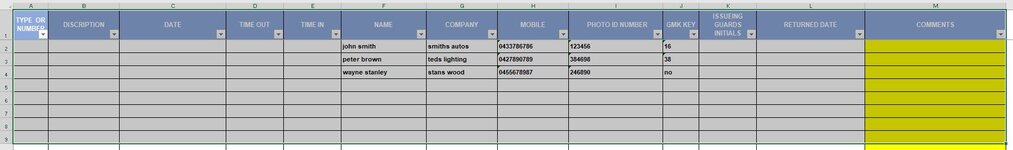
in my work book 1 have 5 columns column F is NAME column G is COMPANY column H is MOBILE NO column I is ID NUMBER column J is KEY NO What i am trying to do is when i type in a name into a cell in the name column the other info autofils into the other columns in rows the columns A TO E Will be filled out manually

 

[Grahamscown]

Copy of Book1TESTER.xlsx
	I
9
Sheet2

 

[Grahamscown]

Copy of Book1TESTER.xlsx
	A	B	C	D	E
1	NAME	COMPANY	MOBILE	PHOTO ID NUMBER	GMK KEY
2	AAA	ABC1	0433709111	12345	26
3	BBB	ABC2	0433709112	12346	28
4	AAA	ABC3	0433709113	12347	30
5	BBB	ABC4	0433709114	12348	32
6	AAA	ABC5	0433709115	12349	34
7	BBB	ABC6	0433709116	12350	36
8	AAA	ABC7	0433709117	12351	38
9	BBB	ABC8	0433709118	12352	40
10	AAA	ABC9	0433709119	12353	42
11	BBB	ABC10	0433709120	12354	44
12	AAA	ABC11	0433709121	12355	46
13	BBB	ABC12	0433709122	12356	48
14	AAA	ABC13	0433709123	12357	50
15	BBB	ABC14	0433709124	12358	52
16
17
18
19
20
21
22
23
24
25
26
27
28
29
30
31
Sheet1

 

[Grahamscown]

is thhat done ok
i can find upload image but not mini file

 

[maabadi]

Yes. For Destination Sheet also upload.
First select range. Then click on minisheet.
Click oK on message box and then paste here.

 

[Grahamscown]

Yes. For Destination Sheet also upload.
First select range. Then click on minisheet.
Click oK on message box and then paste here.

Copy of Book1TESTER.xlsx
	A	B	C	D	E	F	G	H	I	J	K	L	M
1	TYPE OR NUMBER	DISCRIPTION	DATE	TIME OUT	TIME IN	NAME	COMPANY	MOBILE	PHOTO ID NUMBER	GMK KEY	ISSUEING GUARDS INITIALS	RETURNED DATE	COMMENTS
2						AAA	=IFERROR(VLOOKUP($F9,Sheet1!$A:$E,COLUMNS(Sheet2!$F$1:I$1),FALSE),"")
3						BBB
4						BBB	ABC2
5						BBB	ABC2
6
7
8
9
10
11
12
13
14
15
16
17
18
19
20
21
22
23
24
25
26
27
28
29
30
31
32
33
34
35
36
37
38
39
40
41
Sheet2

Cell Formulas
Range	Formula
D27	D27	=IFERROR(VLOOKUP($F9,Sheet1!$A:$E,COLUMNS(Sheet2!$F$1:I$1),FALSE),"")

 

[maabadi]

Why Change my formula at G2 if your source data is in Sheet1 Columns A to G
Paste this formula at G2

 =IFERROR(VLOOKUP($F2,Sheet1!$A:$E,COLUMNS(Sheet2!$F$1:G$1),FALSE),"")

And Press ENTER
THEN
Drag it to Cell J2 and then drag all of 4 cells until last row of tables (don't Care column G filled or Empty)

 

[Grahamscown]

Why Change my formula at G2 if your source data is in Sheet1 Columns A to G
Paste this formula at G2

 =IFERROR(VLOOKUP($F2,Sheet1!$A:$E,COLUMNS(Sheet2!$F$1:G$1),FALSE),"")

And Press ENTER
THEN
Drag it to Cell J2 and then drag all of 4 cells until last row of tables (don't Care column G filled or Empty)

Copy of Book1TESTER.xlsx
	G	H	I	J
2	=IFERROR(VLOOKUP($F2,Sheet1!$A:$E,COLUMNS(Sheet2!$F$1:G$1),FALSE),"")	=IFERROR(VLOOKUP($F2,Sheet1!$A:$E,COLUMNS(Sheet2!$F$1:G$1),FALSE),"")	=IFERROR(VLOOKUP($F2,Sheet1!$A:$E,COLUMNS(Sheet2!$F$1:G$1),FALSE),"")	=IFERROR(VLOOKUP($F2,Sheet1!$A:$E,COLUMNS(Sheet2!$F$1:G$1),FALSE),"")
Sheet2

 

[Grahamscown]

Copy of Book1TESTER.xlsx
	G	H	I	J
2	=IFERROR(VLOOKUP($F2,Sheet1!$A:$E,COLUMNS(Sheet2!$F$1:G$1),FALSE),"")	=IFERROR(VLOOKUP($F2,Sheet1!$A:$E,COLUMNS(Sheet2!$F$1:G$1),FALSE),"")	=IFERROR(VLOOKUP($F2,Sheet1!$A:$E,COLUMNS(Sheet2!$F$1:G$1),FALSE),"")	=IFERROR(VLOOKUP($F2,Sheet1!$A:$E,COLUMNS(Sheet2!$F$1:G$1),FALSE),"")
Sheet2

Copy of Book1TESTER.xlsx
	A	B	C	D	E	F	G	H	I	J	K	L	M
1	TYPE OR NUMBER	DISCRIPTION	DATE	TIME OUT	TIME IN	NAME	COMPANY	MOBILE	PHOTO ID NUMBER	GMK KEY	ISSUEING GUARDS INITIALS	RETURNED DATE	COMMENTS
2							=IFERROR(VLOOKUP($F2,Sheet1!$A:$E,COLUMNS(Sheet2!$F$1:G$1),FALSE),"")	=IFERROR(VLOOKUP($F2,Sheet1!$A:$E,COLUMNS(Sheet2!$F$1:G$1),FALSE),"")	=IFERROR(VLOOKUP($F2,Sheet1!$A:$E,COLUMNS(Sheet2!$F$1:G$1),FALSE),"")	=IFERROR(VLOOKUP($F2,Sheet1!$A:$E,COLUMNS(Sheet2!$F$1:G$1),FALSE),"")
3
4
5
6
7
8
Sheet2

 

[maabadi]

Are you know how to drag formula?
You copied my formula at all cells at row 2 (Not Dragged).
Change your calculation at automatic also.
When you input data at column F then you see result at other cells.

 

[maabadi]

And One other Things I understand, Why you have repeated data at Name Column at Source sheet? (Based Post #12)
Then How We know which one should be filled at Other Columns.
Vlookup work based Unique items at Name Column.
With Unique Item at Column Name at Sheet1 this is example file I uploaded. See Sheet2 to view Results:
Test1.xlsx