-
If you would like to post, please check out the MrExcel Message Board FAQ and register here. If you forgot your password, you can reset your password.
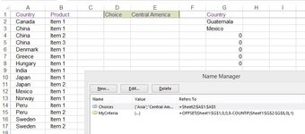
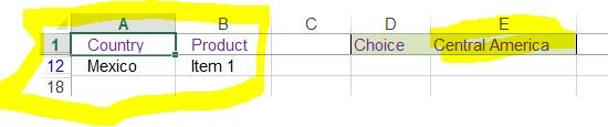
Auto-Filters with Criteria Ranges Stored in Rows
- Thread starter Saighead
- Start date
Similar threads
- Question


