Autofilter at row 4 and copy filtered visible rows from 6 and futher on

[DirkPH]

Hi All,

I am struggling to get certain rows copied from sheet "Data" into another workbook with autofilter.

I want to autofilter --> row 4 --> field 170 --> "<>" --> and copy all visible lines starting from row 5. Then I want to paste these visible lines as value into another workbook also at row 5.
Preferably there should not be any limitation regarding the rows.

Do you have any suggestions?

Thank you!
BR, Dirk

 

[JW00]

Hi, in the following code you will have to change the bold font in these lines;

Sheets("Data").Range("A4").AutoFilter Field:=3, Criteria1:="=*03", Operator:=xlAnd

Workbooks.Open Filename:="M:\Filtered Results.xlsx"

Set rng3 = Sheets("Sheet1").Range(Cells(5, 1), Cells(j, k))

Sub FilteredArrayToWorkbook()
Dim c As Range, rng As Range, rng1 As Range, rng2 As Range, rng3 As Range
Dim i As Long, j As Long, k As Long, m As Long, n As Long
Dim arr() As String, arr1() As Variant, arr2() As Variant
Dim s As String, t As String
Dim AC As Long, LR As Long, LC As Long, RN As Long

    Application.ScreenUpdating = False
    Application.DisplayAlerts = False
    
    Sheets("Data").Range("A4").AutoFilter Field:=3, Criteria1:="=*03", Operator:=xlAnd
    
    Sheets("Data").Range("A4").CurrentRegion.Select

    AC = ActiveCell.Column
    RN = ActiveCell.Row
    LR = ActiveSheet.Cells(ActiveSheet.Rows.Count, AC).End(xlUp).Row
    LC = ActiveCell.CurrentRegion.Columns.Count
    Set rng = Range(Cells(RN + 1, AC), Cells(LR, AC))
    Set rng1 = Range(Cells(RN + 1, AC), Cells(LR, LC))
    arr1 = rng1.Value
    j = 0
    For Each c In rng
        If Not c.Rows.Hidden Then
            j = j + 1
            s = s & c.Row & ", "
        End If
    Next c
    
    arr = Split(s, ", ")
    
    Set rng2 = Range(Cells(RN, AC), Cells(UBound(arr) + RN - 1, LC + AC - 1))
    
    arr2 = rng2.Value
    
    m = 1
    n = 0
    For i = LBound(arr1) To UBound(arr1)
        For k = n To UBound(arr) - 1
            For j = LBound(arr1, 2) To UBound(arr1, 2)
                If arr(n) = i + RN - 1 Then
                   arr2(m, j) = arr1(i, j)
                Else
                   GoTo Skip
                End If
            Next j
        Next k
        m = m + 1
        n = n + 1
Skip:
    Next i
    
    j = UBound(arr2)
    k = UBound(arr2, 2)
    
    Workbooks.Open Filename:="M:\Filtered Results.xlsx"

    Set rng3 = Sheets("Sheet1").Range(Cells(5, 1), Cells(j, k))
    rng3.Value = arr2
    
    Application.ScreenUpdating = True
    Application.DisplayAlerts = True

End Sub

 

[DirkPH]

Hi JW00,

Great effort. Your code is almost working. It copies all filtered lines including 2 lines (?) above the header. Unfortunately it does not paste all lines in my cuurent sheet. At the bottom it misses 3 lines. Do you have any idea how this can happen? See below my code which I had to adjust to my situation.

I have second sheet "Data-M"where I want to do exactly the same and paste data to the same sheet on the end of previous macro. I changed coding to Sheet to "Data-M", but it gives an error for the bold line in below code. I do not understand because source the is exactly identical. Are you able to support me?

Thank you in advance!


Sub DataM()
Dim c As Range, rng As Range, rng1 As Range, rng2 As Range, rng3 As Range
Dim i As Long, j As Long, k As Long, m As Long, n As Long
Dim arr() As String, arr1() As Variant, arr2() As Variant
Dim s As String, t As String
Dim AC As Long, LR As Long, LC As Long, RN As Long

Application.ScreenUpdating = False
Application.DisplayAlerts = False

Dim sourceworkbook As Workbook
Dim currentworkbook As Workbook

Set currentworkbook = ThisWorkbook
Set sourceworkbook = Workbooks.Open("https://parkercorp.sharepoint.com/sites/BusinessManagementSystem159/Shared Documents/Test/Kaizen/2. Shop floor - Orders.xlsm")

Sheets("Data").Activate
ActiveSheet.Unprotect "vst"

sourceworkbook.Activate
Sheets("Data").Range("A4").AutoFilter Field:=170, Criteria1:="<>", Operator:=xlAnd

Sheets("Data").Range("A4").CurrentRegion.Select

AC = ActiveCell.Column
RN = ActiveCell.Row
LR = ActiveSheet.Cells(ActiveSheet.Rows.Count, AC).End(xlUp).Row
LC = ActiveCell.CurrentRegion.Columns.Count
Set rng = Range(Cells(RN + 1, AC), Cells(LR, AC))
Set rng1 = Range(Cells(RN + 1, AC), Cells(LR, LC))
arr1 = rng1.Value
j = 0
For Each c In rng
If Not c.Rows.Hidden Then
j = j + 1
s = s & c.Row & ", "
End If
Next c

arr = Split(s, ", ")

Set rng2 = Range(Cells(RN, AC), Cells(UBound(arr) + RN - 1, LC + AC - 1))

arr2 = rng2.Value

m = 1
n = 0
For i = LBound(arr1) To UBound(arr1)
For k = n To UBound(arr) - 1
For j = LBound(arr1, 2) To UBound(arr1, 2)
If arr = i + RN - 1 Then
arr2(m, j) = arr1(i, j)
Else
GoTo Skip
End If
Next j
Next k
m = m + 1
n = n + 1
Skip:
Next i

j = UBound(arr2)
k = UBound(arr2, 2)


currentworkbook.Activate
Worksheets("Data").Activate

Set rng3 = Sheets("Data").Range(Cells(5, 1), Cells(j, k))
rng3.Value = arr2

Application.ScreenUpdating = True
Application.DisplayAlerts = True

 

[JW00]

My apologies for that, I'd adapted it from something else, it should now extract the correct rows & regarding the error that usually errors if you are not on that sheet, I would step through the code using F8 & see what sheet you are on at that point, I added shn = "Data" at the top, so shn replaces "Data" in the rest of the code so you only have to change it once. Add your additions to the new code & see how you get on.

Sub Data()
Dim c As Range, rng As Range, rng1 As Range, rng2 As Range, rng3 As Range
Dim i As Long, j As Long, k As Long, m As Long, n As Long
Dim arr() As String, arr1() As Variant, arr2() As Variant
Dim s As String, t As String, shn As String
Dim AC As Long, LR As Long, LC As Long, RN As Long

    Application.ScreenUpdating = False
    Application.DisplayAlerts = False
    
    shn = "Data"
    
    Sheets(shn).Range("A4").AutoFilter Field:=3, Criteria1:="=*03", Operator:=xlAnd
    
    Sheets(shn).Range("A4").CurrentRegion.Select

    AC = ActiveCell.Column
    RN = ActiveCell.Row
    LR = ActiveSheet.Cells(ActiveSheet.Rows.Count, AC).End(xlUp).Row
    LC = ActiveCell.CurrentRegion.Columns.Count
    Set rng = Range(Cells(RN + 1, AC), Cells(LR, AC))
    Set rng1 = Range(Cells(RN + 1, AC), Cells(LR, LC))
    arr1 = rng1.Value
    j = 0
    For Each c In rng
        If Not c.Rows.Hidden Then
            j = j + 1
            s = s & c.Row & ", "
        End If
    Next c
    
    arr = Split(s, ", ")
    
    Set rng2 = Range(Cells(RN, AC), Cells(UBound(arr) + RN - 1, LC + AC - 1))
    
    arr2 = rng2.Value
    
    m = 1
    n = 0
    For i = LBound(arr1) To UBound(arr1)
            For j = LBound(arr1, 2) To UBound(arr1, 2)
                If arr(n) = i + RN Then
                   arr2(m, j) = arr1(i, j)
                Else
                   GoTo Skip
                End If
            Next j
        m = m + 1
        n = n + 1
Skip:
    Next i
    
    j = UBound(arr2)
    k = UBound(arr2, 2)
    
    Workbooks.Open Filename:="M:\Filtered Results.xlsx"

    Set rng3 = Sheets("Sheet1").Range(Cells(5, 1), Cells(j + 4, k))
    rng3.Value = arr2
    
    Application.ScreenUpdating = True
    Application.DisplayAlerts = True

End Sub

 

[DirkPH]

Great! It did the trick, thank you very much. It still selects the 2 rows above the header as well, but it looks okay. I have also fixed the error for the second data extract.

Question: I want to add this second data extract under the first data extract. I have used the code "Range("A" & Rows.Count).End(xlUp).Offset(1).Select" but this seems like it doesn't do anything good. It pastes the data in the first data set one line lower, see bold section in table below.

Do you have any suggestions? Does the formula alsways copy the header as well?

Besides copy this filtered data and paste it elsewhere, I am also looking for an option to paste copied data in the same area as value. (to remove formulas). Is this code als applicable by just changing the destination?

I am sorry to bother you like this.

BR, Dirk

WO	PF	Product	# P	# M	Date
WO	PF	Product	# P	# M	Date
Testmodule	NX	1212-7--	-	2	31-01-22
Testmodule	NX	1212-7--	-	4	31-01-22
Testmodule	NX	1212-7--	-	1	31-01-22
15900008	ML	3115	2​	4	31-01-22

 

[JW00]

Put the following code in your module & then replace the following lines with the ones in bold letters;

Function LastRowColumn(RowColumn As String) As Long
Dim sht As Worksheet

Set sht = ActiveSheet

Select Case LCase(Left(RowColumn, 1)) 'If they put in 'row' or column instead of 'r' or 'c'.
  Case "c"
    LastRowColumn = sht.Cells.Find("*", LookIn:=xlFormulas, SearchOrder:=xlByColumns, _
    SearchDirection:=xlPrevious).Column
  Case "r"
    LastRowColumn = sht.Cells.Find("*", LookIn:=xlFormulas, SearchOrder:=xlByRows, _
    SearchDirection:=xlPrevious).Row
  Case Else
    LastRowColumn = 1
End Select

End Function

Sheets(shn).Range("A4").CurrentRegion.Select
Sheets(shn).Range("A4")..Select

LR = ActiveSheet.Cells(ActiveSheet.Rows.Count, AC).End(xlUp).Row
LR = LastRowColumn("R")

LC = ActiveCell.CurrentRegion.Columns.Count
LC = LastRowColumn("C")

You can also use LR = LastRowColumn("R") +1 to get your next empty row.

If you want to paste data over itself to remove formulas, personally I would do that manually, ctrlA to select all data, copy & paste values.

 

[DirkPH]

Hi JW00,

I am not sure how to implement this. It doesn't allow me to add this code to the existing module?
Sorry, I am not familiar with function statements.

 

[JW00]

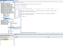
No problem, the "Function" code is written below the "End Sub" or "End Function" of any previous code, a vba "Function" is just like the backend of a worksheet formula. It works the same way as a formula in that you pass it the parameters & it returns your requirement, some are written to be called in vba, some are written to be called from the formula bar on the worksheet & some operate on both plains. This function for getting the last row or last column, so it is a generally useful function that you are likely to use in future projects, therefore personally I would insert a new module into your workbook & place the code in there, you can then rename the module in the property window to something like "mdLastRowColumn", then if you right click the module & export it, that way you can just import it back into any future project (see screenshot).

To use the function, firstly select the top left cell of your range (eg "Sheets("Sheet1").Range("A4").Select"), then write the variable to which you wish to assign the value to, followed by an equals sign & then the function itself (see example), the "R" refers to row & type "C" for the column.


Variable Name = LastRowColumn("R")

I hope that helps, if you have any problems you can always upload a mini version of your workbook (remove any personal data) to google drive & I will take a look & get it working & repost it for you to download.

 

[DirkPH]

Hi JA00,

Thanks for your help. While trying I am getting the same error as earlier;

See below images of my files. The source files (Data_P en Data_T) are identical and filtered for non empty rows in column 172. The results I want to copy in the currentworkbook below each other with Data_P on top. Ideally the currentworkook should first be cleared starting from row 5. It is not a must because the rows will be more and more, but it would be then perfect.

To complete the picture I have added at the bottom of this message actual code as well .

Thank you


This is the currentworkbook

This is the source workbook;

Actual code:



Sub DataP()


Dim c As Range, rng As Range, rng1 As Range, rng2 As Range, rng3 As Range
Dim i As Long, j As Long, k As Long, m As Long, n As Long
Dim arr() As String, arr1() As Variant, arr2() As Variant
Dim s As String, t As String, shn As String
Dim AC As Long, LR As Long, LC As Long, RN As Long

Application.ScreenUpdating = False
Application.DisplayAlerts = False

Dim sourceworkbook As Workbook
Dim currentworkbook As Workbook

Set currentworkbook = ThisWorkbook
Set sourceworkbook = Workbooks.Open("https://parkercorp.sharepoint.com/sites/BusinessManagementSystem159/Shared Documents/Test/Kaizen/2. Shop floor - Orders.xlsm")

ThisWorkbook.Sheets("Data").Activate
ActiveSheet.Unprotect "vst"

shn = "Data_P"

sourceworkbook.Activate
Sheets(shn).Range("A4").AutoFilter Field:=172, Criteria1:="<>", Operator:=xlAnd

Sheets(shn).Range("A4").Select

AC = ActiveCell.Column
RN = ActiveCell.Row
LR = LastRowColumn("R")
LC = LastRowColumn("C")
Set rng = Range(Cells(RN + 1, AC), Cells(LR, AC))
Set rng1 = Range(Cells(RN + 1, AC), Cells(LR, LC))
arr1 = rng1.Value
j = 0
For Each c In rng
If Not c.Rows.Hidden Then
j = j + 1
s = s & c.Row & ", "
End If
Next c

arr = Split(s, ", ")

Set rng2 = Range(Cells(RN, AC), Cells(UBound(arr) + RN - 1, LC + AC - 1))

arr2 = rng2.Value

m = 1
n = 0
For i = LBound(arr1) To UBound(arr1)
For j = LBound(arr1, 2) To UBound(arr1, 2)
If arr = i + RN Then
arr2(m, j) = arr1(i, j)
Else
GoTo Skip
End If
Next j
m = m + 1
n = n + 1
Skip:
Next i

j = UBound(arr2)
k = UBound(arr2, 2)

currentworkbook.Activate
Worksheets("Data").Activate


Set rng3 = Sheets("Data").Range(Cells(5, 1), Cells(j + 4, k))
rng3.Value = arr2

Application.ScreenUpdating = True
Application.DisplayAlerts = True





End Sub

 

[JW00]

I have been through the code & changed the approach to avoid that line of code entirely, I have placed all the changes in your code from above, I am pasting the code in one complete block, If you had put the "LastRowColumn" in another module, just delete it as it will be repeated.

Sub DataP()
Dim c As Range, rng As Range, rng1 As Range, rng2 As Range, rng3 As Range
Dim i As Long, j As Long, k As Long, m As Long, n As Long
Dim arr() As String, arr1() As Variant, arr2() As Variant
Dim s As String, t As String, shn As String
Dim AC As Long, LR As Long, LC As Long, RN As Long

Application.ScreenUpdating = False
Application.DisplayAlerts = False

Dim sourceworkbook As Workbook
Dim currentworkbook As Workbook

Set currentworkbook = ThisWorkbook
Set sourceworkbook = Workbooks.Open("https://parkercorp.sharepoint.com/sites/BusinessManagementSystem159/Shared Documents/Test/Kaizen/2. Shop floor - Orders.xlsm")

ThisWorkbook.Sheets("Data").Activate
ActiveSheet.Unprotect "vst"

shn = "Data_P"

sourceworkbook.Activate
Sheets(shn).Range("A4").AutoFilter Field:=172, Criteria1:="<>", Operator:=xlAnd

AC = 1
RN = GetFilteredRangeTopRow
LR = GetFilteredRangeBottomRow
LC = LastRowColumn("C")
Set rng = Range(Cells(RN, AC), Cells(LR, AC))
Set rng1 = Range(Cells(RN, AC), Cells(LR, LC))
arr1 = rng1.Value
j = 0
For Each c In rng
If Not c.Rows.Hidden Then
j = j + 1
s = s & c.Row & ", "
End If
Next c

arr = Split(s, ", ")

Set rng2 = Range(Cells(RN, AC), Cells(UBound(arr) + RN, LC))

arr2 = rng2.Value

m = 1
n = 0
For i = LBound(arr1) To UBound(arr1)
For j = LBound(arr1, 2) To UBound(arr1, 2)
If arr(n) = i + RN - 1 Then
arr2(m, j) = arr1(i, j)
Else
GoTo Skip
End If
Next j
m = m + 1
n = n + 1
Skip:
Next i

j = UBound(arr2)
k = UBound(arr2, 2)

currentworkbook.Activate
Worksheets("Data").Activate

Set rng3 = Sheets("Data").Range(Cells(5, 1), Cells(j + 4, k))
rng3.Value = arr2

Application.ScreenUpdating = True
Application.DisplayAlerts = True

End Sub


Function LastRowColumn(RowColumn As String) As Long
Dim sht As Worksheet

Set sht = ActiveSheet

Select Case LCase(Left(RowColumn, 1)) 'If they put in 'row' or column instead of 'r' or 'c'.
  Case "c"
    LastRowColumn = sht.Cells.Find("*", LookIn:=xlFormulas, SearchOrder:=xlByColumns, _
    SearchDirection:=xlPrevious).Column
  Case "r"
    LastRowColumn = sht.Cells.Find("*", LookIn:=xlFormulas, SearchOrder:=xlByRows, _
    SearchDirection:=xlPrevious).Row
  Case Else
    LastRowColumn = 1
End Select

End Function


Function GetFilteredRangeTopRow() As Long
  Dim HeaderRow As Long, LastFilterRow As Long
  On Error GoTo NoFilterOnSheet
  With ActiveSheet
    HeaderRow = .AutoFilter.Range(1).Row
    LastFilterRow = .Range(Split(.AutoFilter.Range.Address, ":")(1)).Row
    GetFilteredRangeTopRow = .Range(.Rows(HeaderRow + 1), .Rows(Rows.Count)). _
                                    SpecialCells(xlCellTypeVisible)(1).Row
    If GetFilteredRangeTopRow = LastFilterRow + 1 Then GetFilteredRangeTopRow = 0
  End With
NoFilterOnSheet:
End Function
 
Function GetFilteredRangeBottomRow() As Long
  Dim HeaderRow As Long, LastFilterRow As Long, Addresses() As String
  On Error GoTo NoFilterOnSheet
  With ActiveSheet
    HeaderRow = .AutoFilter.Range(1).Row
    LastFilterRow = .Range(Split(.AutoFilter.Range.Address, ":")(1)).Row
    Addresses = Split(.Range((HeaderRow + 1) & ":" & LastFilterRow). _
                      SpecialCells(xlCellTypeVisible).Address, "$")
    GetFilteredRangeBottomRow = Addresses(UBound(Addresses))
  End With
NoFilterOnSheet:
End Function