Automatically Update Code

[riedyp]

I have a code that changes the range of data for a chart as more values are entered. I want the user to enter their values and the chart to automatically update but am unsure how to do this. The code works fine when i manually run it, so the only challenge is making it run by itself. Any help would be appreciated.
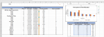
The chart i am having difficulty with is the time spent versus time allocated chart.

Private Sub TimeSpent()
Dim ch As ChartObject
Set ch = Worksheets("Executive Summary").ChartObjects("Chart 8")
LastRow = Worksheets("Executive Summary").Columns("J").Find(1, SearchDirection:=xlPrevious, LookIn:=xlValues, LookAt:=xlWhole).Row

Worksheets("Executive Summary").ChartObjects("Chart 8").Activate


    ActiveChart.FullSeriesCollection(1).Name = Worksheets("Executive Summary").Range("L34")
    ActiveChart.FullSeriesCollection(1).Values = Range(Cells(35, 12), Cells(LastRow, 12))
   ' ActiveChart.FullSeriesCollection(1).GapWidth = 60
    ActiveChart.FullSeriesCollection(2).Name = Worksheets("Executive Summary").Range("M34")
    ActiveChart.FullSeriesCollection(2).Values = Range(Cells(35, 13), Cells(LastRow, 13))

    ActiveChart.HasLegend = True
End Sub

 

[Zack Barresse]

No need for VBA. Define a named range to:

=OFFSET('Executive Summary'!$B$23,,,COUNTA('Executive Summary'!$B$23:$B$1000),6)

Where row 1000 is the largest your data would possibly grow, ensuring nothing is below your data, and assign that named range to your chart series.

 

[riedyp]

Thanks for your response. Just want to clarify that I am working on the chart on the right side of that picture. Will this still work if these cells are dependent on another sheet? Below are the formulas in those cells until row 60. attached is a picture of the sheet the values are being inputted on.
K35: =IF(ROW()-ROW(K$34)<=SUM(IFERROR(--(('Project - Gantt Chart'!$B$9:$B$45/INT('Project - Gantt Chart'!$B$9:$B$45))=1),"")),ROW()-ROW(K$34),"")

L35: =IFERROR(INDEX('Project - Gantt Chart'!$B$9:$I$45,MATCH('Executive Summary'!$K35,'Project - Gantt Chart'!$B$9:$B$45,0),4),"")

M35: =IFERROR(INDEX('Project - Gantt Chart'!$B$9:$I$45,MATCH('Executive Summary'!$K35,'Project - Gantt Chart'!$B$9:$B$45,0),5),"")

N35: =IFERROR(INDEX('Project - Gantt Chart'!$B$9:$I$45,MATCH('Executive Summary'!$K35,'Project - Gantt Chart'!$B$9:$B$45,0),8),"")

 

[Zack Barresse]

It should work. A dynamic named range is one which moves as data moves (grows/shrinks). I'm not sure the formula You would need to create the named range to wherever the series data is plotted from. I'm not entirely sure where that is right now. For the chart in question, can you tell us exactly where the data is located? Other pertinent information would be if there is any adjacent data below/next to it. If you are using Table's, you don't need a dynamic named range, you can just point it to that as a source and it will grow/shrink automatically, although the references you see on the series may show up as A1 style notation.

 

[riedyp]

The data on the "Time Spent"chart is pulled from the "Time Spent" Table below the Chart. The values of the "Time Spent" Table are pulled from another sheet in the workbook that has the user input data into a Gantt Chart Table.(see attached picture) Unfortuantely, the data as it shows up in that Gantt Chart Table would not be in the format i want.
The Time Spent Table only pulls "Phase #'s" that are integers along with that "Phase #'s" "Hours Allocated" "Hours Spent" and "Percent Complete".
To the left of the Time Spent Table there are "1"'s if that row has a value populated. This is how I was tracking the "Last Row" in my code.(can

I am trying for my chart to not show empty values, so that is my challenge with this. Essentially this sheet is supposed to act like a dashboard where the user does not have to edit anything.
Let me know if you need any more clarification. Thanks again for your time and patience.

 

[Zack Barresse]

If your Time Spent data is looking somewhere else and you want to return a blank for that series data point, instead return NA(), which a chart will not plot and so it appears blank. It's hard to elaborate further without knowing the formulas utilized.