Average date ( day & month only ) for the last number of years using a dynamic range

[Tikey]

I use Excel 2019 from the Office Pro package.

I currently use the following formula to average a series of dates for just the day and month:

=ROUNDUP(AVERAGE(IF(ISNUMBER(C8:C38),DATE(1900,MONTH(C8:C38),DAY(C8:C38)))),0) - entered using Ctrl, Shift, Enter

This works fine, but I would like to take this a step further and adapt this to use in a dynamic range to cover the last 10 years.

I have tried editing this using the OFFSET function without any success, I am struggling with this, can anyone offer any suggestions.

Thanks in anticipation.

 

[BSALV]

make a named range of that range and use it in the formula

 

[Tikey]

Thanks for your reply, unfortunately I would need further guidence if possible.

 

[BSALV]

in the ribbon goto formula>define name, as new name give there "MyName" and refers to for example C8:C1000, later you can even make that name dynamic.
your formula

=ROUNDUP(AVERAGE(IF(ISNUMBER(MyName),DATE(1900,MONTH(MyName),DAY(MyName)))),0)

 

[Tikey]

Ok thanks, but I'm still confused, as although the range will be replaced by a named range, my thinking is the formula will still work the same and not dynamically for the last set number of years eg 10.

 

[BSALV]

my range is named "last10" and refers to

=OFFSET(Blad12!$C$8,MAX(0,COUNTA(Blad12!$C$8:$C$60)-10),,10,)

testing.xlsx
	B	C	D	E	F	G	H	I
4
5					=VERSCHUIVING(Blad12!$C$8;MAX(0;AANTALARG(Blad12!$C$8:$C$60)-10);;10;)
6					=OFFSET(Blad12!$C$8,MAX(0,COUNTA(Blad12!$C$8:$C$60)-10),,10,)
7
8		2019
9		2020
10		2021			the last 10		1st cell
11		2022			2026		$C$15
12		2023			2027
13		2024			2028
14		2025			2029
15		2026			2030
16		2027			2031
17		2028			2032
18		2029			2033
19		2030			2034
20		2031			2035
21		2032
22		2033
23		2034
24		2035
25
26
Blad12

Cell Formulas
Range	Formula
F11:F20	F11	=Last10
H11	H11	=CELL("adres",Last10)
Dynamic array formulas.

 

[Tikey]

Thank you for your reply.

Whilst I don't fully understand it, I am wondering if my question wasn't very clear, as I cannot see average in the formula and the answer appears to be the year rather than the day and month.
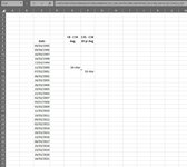
Hopefully the following example will be clearer. Column C shows the dates to be averaged. Cell E13 shows the day / month average of all the data in Column C and Cell F14 the last 10 year ( C25:C34 ) day / month average of the data in Column C, this is the answer I am seeking. But, I wish the spreadsheet to respond dynamically so that when another date is added to C35, the answer in F14 will update automatically to the day /month average of cells C26:C35.

Hopefully I have made the question clearer.

 

[BSALV]

defined name = "mydates" with the formula in D3 without the leading '
columns D and E are only for check, you don't need them later.
G11 = today-10 years = all the dates later then that date are used. If you want it starting 1 january, just change the formula in G11
The value you want is G8, but is G10/G9, the same values as in cells D5:E5, for the check.
So those 2 were also only tempory. You can give G8 the numberformat "dd-mm" for example
Column C is filled with random dates starting 1/1/2010 until 31/12/2021. They change when the worksheet recalculates, so replace them with your fixed dates.

The average for all the dates is

=SUMPRODUCT(DATE(0,MONTH(MyDates),DAY(MyDates)))/COUNT(MyDates)

Map1
	B	C	D	E	F	G	H	I
2
3		mydates	=OFFSET(Blad6!$C$8,,,COUNT(Blad6!$C$8:$C$100),)
4
5			31	7170
6			check	check
7			count	dag
8		7/09/2020	1	251	avg	231,2903226
9		23/01/2010	0	23	count	31
10		11/10/2010	0	285	sum	7170
11		27/06/2016	1	179	min date	16/01/2012
12		28/05/2014	1	149
13		25/04/2012	1	116
14		17/03/2015	1	77
15		23/05/2016	1	144
16		17/07/2014	1	199
17		25/03/2012	1	85
18		2/12/2020	1	337
19		28/12/2015	1	363
Blad6

Cell Formulas
Range	Formula
D5	D5	=SUM(D8:D100)
E5	E5	=SUMPRODUCT((E8:E100),D8:D100)
C8:C19	C8	=DATE(2010,1,RANDBETWEEN(1,12*365))
D8:D19	D8	=--(C8>$G$11)
E8:E19	E8	=DATE(0,MONTH(C8),DAY(C8))
G8	G8	=SUMPRODUCT(DATE(0,MONTH(MyDates),DAY(MyDates))*(MyDates>$G$11))/SUMPRODUCT(--(MyDates>$G$11))
G9	G9	=SUMPRODUCT(--(MyDates>$G$11))
G10	G10	=SUMPRODUCT(DATE(0,MONTH(MyDates),DAY(MyDates))*(MyDates>$G$11))
G11	G11	=EDATE(TODAY(),-10*12)

 

[Tikey]

Thanks again, I think I am slowly understanding your solution.

A couple of questions if I could, what is Blad6! in the formula in D3, what is EDATE for in the G11 formula and how could I change that to 1 January if required ?

 

[Tikey]

Apologies, I replied without thinking, Blad6! will be your sheet name I think.