Average of every 7th cell in a row

[ashleyjmetcalfe]

Hi,

Sorry I have looked at other posts and seem to be incapable of reconciling them. So I would ask someone to take pity on me and write this formula for me!

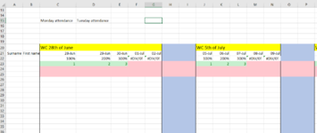
I am trying to do an attendance tracker for school. I want to get an average of every 7th day so i can do monday average, tuesday etc.

Monday's run from C23 to MH23. The average should include 0's but disregard any blank values. (When the register is taken it will be 1 = present, 0= absent. blank cell means it is for a future week!)

Can someone help me please!

Thanks,

Ashley

 

[jasonb75]

Perhaps something like this, array confirmed with Ctrl Shift Enter.

=AVERAGE(IF(WEEKDAY($C$21:$MH$21)=2,$C23:$MH23))

Changing the weekday number according to the day that you want the average for. =2 for Monday through to =6 for Friday.

 

[Snakehips]

@jasonb75 I don't believe the above ignores the blank cells.
I'm not entirely sure if @ashleyjmetcalfe is wanting an average for an individual or for a group of individuals?

Here is another approach that could adapt either way.

MRXLMAY21.xlsm
	A	B	C	D	E	F	G	H	I	J	K	L	M	N	O	P	Q	R	S	T	U	V
11			Mon	Tue	Wed	Thur	Frid
12	Single Line Average		100.00%	50.00%	0
13	Range Average		100.00%	75.00%	50.00%
14
15
16
17
18
19
20
21			28 Jun	29 Jun	30 Jun	01 Jul	02 Jul			05 Jul	06 Jul	07 Jul	08 Jul	09 Jul			12 Jul	13 Jul	14 Jul	15 Jul	16 Jul
22
23			1	1	0	1	1			1	0	0
24			1	1	1	1	1			1	1	1
25
Sheet7 (2)

Cell Formulas
Range	Formula
C12	C12	=IFERROR(SUMPRODUCT((WEEKDAY($C$21:$MH$21)=2)*($C23:$MH23))/SUMPRODUCT((WEEKDAY($C$21:$MH$21)=2)*(ISNUMBER($C23:$MH23))),"")
D12	D12	=IFERROR(SUMPRODUCT((WEEKDAY($C$21:$MH$21)=3)*($C23:$MH23))/SUMPRODUCT((WEEKDAY($C$21:$MH$21)=3)*(ISNUMBER($C23:$MH23))),"")
E12	E12	=IFERROR(SUMPRODUCT((WEEKDAY($C$21:$MH$21)=4)*($C23:$MH23))/SUMPRODUCT((WEEKDAY($C$21:$MH$21)=4)*(ISNUMBER($C23:$MH23))),"")
C13	C13	=IFERROR(SUMPRODUCT((WEEKDAY($C$21:$MH$21)=2)*($C23:$MH33))/SUMPRODUCT((WEEKDAY($C$21:$MH$21)=2)*(ISNUMBER($C23:$MH33))),"")
D13	D13	=IFERROR(SUMPRODUCT((WEEKDAY($C$21:$MH$21)=3)*($C23:$MH33))/SUMPRODUCT((WEEKDAY($C$21:$MH$21)=3)*(ISNUMBER($C23:$MH33))),"")
E13	E13	=IFERROR(SUMPRODUCT((WEEKDAY($C$21:$MH$21)=4)*($C23:$MH33))/SUMPRODUCT((WEEKDAY($C$21:$MH$21)=4)*(ISNUMBER($C23:$MH33))),"")

Hope that helps.

 

[ashleyjmetcalfe]

Thanks for that!

 

[jasonb75]

@jasonb75 I don't believe the above ignores the blank cells.

Good point, but an easy fix

=AVERAGE(IF(WEEKDAY($C$21:$MH$21)=2,IF(ISNUMBER($C23:$MH23),$C23:$MH23)))