Average of Last x Instances of a Criteria

[whothemannow]

Hi all,

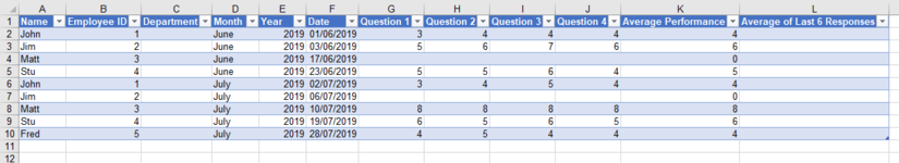
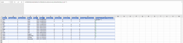
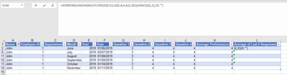
I am working on a spreadsheet about employee performance, with columns of employee name, month, year, performance, etc. (as a result, employees have multiple rows as the data is sorted by dates). How can I calculate the average of each employee's last 6 performance scores (excluding zeroes)? (so that each row would return that employee's average) I have tried numerous formulas and initially thought that I should use AVERAGEIF, but I can't seem to figure it out.
Any help would be greatly appreciated!

 

[Toadstool]

Hi Whothemannow,

With 365 you've more options but here's my approach using Excel 2016.

NOTE: It's probably easier to extract the last 6 (or nth if less than 6 exist) and do an average of those).

Whothemannow.xlsx
	A	B	C	D	E	F	G
1	Name	Date	Performance		Who	Start	Average
2	Fred	01-Jan-02	1		Jim	$A$7	2.833333
3	Sue	30-Nov-02	2			$C$7
4	Jim	29-Oct-03	3
5	Jim	26-Sep-04	0
6	Sue	25-Aug-05	5
7	Jim	24-Jul-06	4
8	Fred	22-Jun-07	4
9	Jim	20-May-08	4
10	Jim	18-Apr-09	3
11	Fred	17-Mar-10	3
12	Jim	13-Feb-11	2
13	Jim	12-Jan-12	2
14	Fred	10-Dec-12	1
15	Jim	08-Nov-13	2
16
Sheet1

Cell Formulas
Range	Formula
G2	G2	=AVERAGEIF(INDIRECT(F2&":$A$99999"),$E$2,INDIRECT($F$3&":$C$99999"))
F2	F2	=ADDRESS(AGGREGATE(14,6,ROW($A$2:$A$99999)-ROW($A$1)/(($A$2:$A$99999=$E$2)*($C$2:$C$99999<>0)),MIN(6,COUNTIF($A$2:$A$99999,$E$2)))+ROW($A$1),COLUMN($A$1))
F3	F3	=ADDRESS(ROW(INDIRECT(F2)),COLUMN($C$2))

 

[Toadstool]

...as I said it's probably easiest to extract the last 6

Whothemannow.xlsx
	A	B	C	D	E	F	G
1	Name	Date	Performance		Who	Last 6	Average
2	Fred	01-Jan-02	1		Jim	2	2.833333
3	Sue	30-Nov-02	2			2
4	Jim	29-Oct-03	3			2
5	Jim	26-Sep-04	0			3
6	Sue	25-Aug-05	5			4
7	Jim	24-Jul-06	4			4
8	Fred	22-Jun-07	4
9	Jim	20-May-08	4
10	Jim	18-Apr-09	3
11	Fred	17-Mar-10	3
12	Jim	13-Feb-11	2
13	Jim	12-Jan-12	2
14	Fred	10-Dec-12	1
15	Jim	08-Nov-13	2
Sheet1 (2)

Cell Formulas
Range	Formula
G2	G2	=AVERAGE(F2:F7)
F2:F7	F2	=IFERROR(INDEX($C$2:$C$99999,AGGREGATE(14,6,ROW($A$2:$A$99999)-ROW($A$1)/(($A$2:$A$99999=$E$2)*($C$2:$C$99999<>0)),ROW()-ROW($F$1))),"")

 

[Fluff]

Another option

+Fluff 1.xlsm
	A	B	C	D
1	Name	Date	Performance
2	Fred	26/05/1989	3
3	Sue	06/06/1989	6
4	Jim	13/09/1993	1
5	Jim	17/11/1993	7
6	Sue	11/08/1994	1
7	Jim	04/06/1995	6
8	Fred	04/04/1996	2
9	Jim	20/03/1998	10
10	Jim	12/07/1998	5
11	Fred	22/01/1999	5
12	Jim	19/04/1999	4	5.50
13	Jim	12/06/1999	1	5.50
14	Fred	28/03/2007	3
15	Jim	23/01/2009	4	5.00
16	Fred	17/12/2010	6
17	Sue	07/09/2011	6
18	Jim	11/04/2013	1	4.17
19	Jim	22/08/2013	1	2.67
20	Sue	02/10/2014	2
21	Jim	28/05/2015	5	2.67
22	Fred	14/06/2015	7	4.33
23	Jim	14/11/2015	6	3.00
24	Jim	01/01/2016	9	4.33
25	Fred	20/12/2017	8	5.17
26	Jim	06/02/2018	3	4.17
27	Jim	04/08/2019	5	4.83
28	Fred	20/06/2020	8	6.17
29	Jim	26/02/2021	3	5.17
Master

Cell Formulas
Range	Formula
D2:D29	D2	=IFERROR(SUM(INDEX(SORT(FILTER(B$2:C2,A$2:A2=A2),1,-1),SEQUENCE(6),2))/6,"")

 

[whothemannow]

Hi guys,

Thanks for the replies. Unfortunately, they do not exactly fit my needs as they are currently, so I thought some greater elaboration would be required. Attached is a screenshot of a construction of a sample table similar to what I currently have. Essentially, I am looking for column L to return that specific employee's average of their last 6 average performance scores excluding zeroes (not necessarily a rolling average). So L2 should be the average of John's overall last 6 average scores regardless of what the month or year is (of course in the actual table there are more months and years). This won't be used for employee specific insights, so it's not feasible to extract the last 6 responses separately for each employee.

I thought about adding a helper column (maybe COUNTIF) to return whether that month's Average Performance for that employee is one of their most recent 6. I thought this would make the averaging easier, rather than having everything in 1 formula, but I wasn't quite able to wrap my head around that either.
Note that I have Office 365 (not sure whether this makes a difference or not).
Thanks in advance!

 

[Fluff]

What should happen if there aren't 6 scores to average?

 

[whothemannow]

What should happen if there aren't 6 scores to average?

Ideally then it would just return either a zero or blank value

 

[Fluff]

In that case how about

=IFERROR(SUM(INDEX(FILTER(K$2:K2,A$2:A2=A2),SEQUENCE(6),2))/6,"")

 

[whothemannow]

In that case how about

=IFERROR(SUM(INDEX(FILTER(K$2:K2,A$2:A2=A2),SEQUENCE(6),2))/6,"")

Hmm, that doesn't seem to work unfortunately, despite John having 6 responses

 

[Fluff]

Change the 2 after the sequence to 1