Averageifs with conditions

[Evendis]

Hi All,

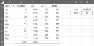
I do have a 5 column spreadsheet. the first is the month of the year, the 2nd to the 5th column has some labels and data. from January to September, I want to average them all. However, I have 2 conditions for column 2 and 3.
I have set 2 cells of the data board and for the 1st cell I want to average if > than a certain % and for the second column a specific number, I want to average all columns . If one or wo of those of selection cells are blank I want the columns to simply average it. if 2 of those columns are blank then average all column. I have used this formula for one single cell : =AVERAGEIFS(B2:B10,C2:C10,">"&G3) and for the columns who are not linked to a selection just average based on the selection.

So, to recap, I want the average of B,C,D,E based on if G3 or H3 has data on both or one only one of those or on none of those, to get the accurate average on cells B11, C 11, D11 and E11. I want to be able to change cell G3 and H3 even delete them to get the full average on each cells on rows 11.

Can you help me adding the correct formula on B11, C11, D11 & E11 cells please.

Thank you very much for your help.
Evendis.

 

[jasonb75]

Unless I'm missing something,

=AVERAGEIFS(B2:B10,C2:C10,">="&N(G3))

should work as long as there are no negative values in the table.

 

[Evendis]

Unless I'm missing something,

=AVERAGEIFS(B2:B10,C2:C10,">="&N(G3))

should work as long as there are no negative values in the table.

It doesn't work. to recap I need the correct formula on B11, C11, D11 & E11 cells. It's a 2 Averageifs formulas with 4 conditions: if both G3 and H3 have data, if only G3 have data, if only H3 has data and finally if both are blank. I need the average on all B11, C11, D11 & E11 cells based or not on G3 and or H3 conditions.

Can you help me ?

 

[jasonb75]

It doesn't work.

It does work, whether or not it gives the results that you expect is something completely different. Your post contains a lot of information with little clarity, the answer that I provided was only as good as that.

You show one existing formula in your question, on which my suggestion was based, without more examples a lot is open to individual interpretation. There is nothing shown to relate G3 and H3 to D11 and E11. If you want a better answer, ask a better question.

Try posting your example using XL2BB, remember to include the expected results based on the sample provided.

 

[Eric W]

Try:

Book1 (version 1).xlsb
	A	B	C	D	E	F	G	H
1	MONTHS	AGENTS	SVL	AHT	NCH
2	Jan	9	90%	900	190		SVL	AGENTS
3	Feb	11	87%	855	221		80%	20
4	Mar	20	75%	795	230
5	Apr	13	62%	911	255
6	May	15	53%	950	311
7	Jun	21	86%	729	245
8	Jul	22	79%	820	271
9	Aug	17	20%	855	332
10	Sep	17	21%	876	364
11		21.0	86.0%	729.0	245.0
Sheet29

Cell Formulas
Range	Formula
B11:E11	B11	=AVERAGEIFS(B2:B10,$B2:$B10,">="&N($H$3),$C$2:$C$10,">="&N($G$3))

 

[Evendis]

Try:

Book1 (version 1).xlsb
	A	B	C	D	E	F	G	H
1	MONTHS	AGENTS	SVL	AHT	NCH
2	Jan	9	90%	900	190		SVL	AGENTS
3	Feb	11	87%	855	221		80%	20
4	Mar	20	75%	795	230
5	Apr	13	62%	911	255
6	May	15	53%	950	311
7	Jun	21	86%	729	245
8	Jul	22	79%	820	271
9	Aug	17	20%	855	332
10	Sep	17	21%	876	364
11		21.0	86.0%	729.0	245.0
Sheet29

Cell Formulas
Range	Formula
B11:E11	B11	=AVERAGEIFS(B2:B10,$B2:$B10,">="&N($H$3),$C$2:$C$10,">="&N($G$3))

Thanks Eric for your help, I really appreciate. We are almost there. We I put on G3 80%, SVL, then all columns average, however when I add on H3 17 (Agents), B11, D11 and E11 do not average. Can you help me please ?

 

[Eric W]

What is your expected result? If you put in 80% and 17, then the only row that satisfies BOTH conditions is row 7, which is what the formula gives you. Or do you want a formula where EITHER condition is true?

 

[Evendis]

Thanks Eric for your help, I really appreciate. We are almost there. We I put on G3 80%, SVL, then all columns average, however when I add on H3 17 (Agents), B11, D11 and E11 do not average. Can you help me please ?

Apologizes, I forgot one single $ in my formula. It looks like it works !!! Thanks a lot Eric for your help.

 

[Eric W]

Glad we could help!

 

[Evendis]

Glad we could help!

Love you Eric for your help, Thank you so much !!!