Averaging letter grades that convert to numbers for a point total

[mpmachala]

I finally figured out how to get a letter grade to equal a point value and average. However I can't figure out the formula to do the same thing, but with data from other columns for a "final grade" as a numerical value.

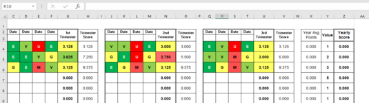
Example, I need C4:F4, J4:M4, and Q4:T4 (some times there won't be a grade in the cell) all to average in column X, but with a numeric value instead.

Letter Grade values:
"E"=4
"V"=3.5
"G"=3
"M"=2
"U"=1

For the life of me, I can't figure out why I can't average across disconnected columns?
Thanks,
Mike

 

[BigBeachBananas]

Look like you have grades for each trimester already. Why don't you just do the average of the trimester grades?
In Z4:

=AVERAGE(H4,O4,V4)

Autofill down

 

[mpmachala]

Look like you have grades for each trimester already. Why don't you just do the average of the trimester grades?
In Z4:

=AVERAGE(H4,O4,V4)

Autofill down

Yeah, my brain was so fried from figuring out the rest, I didn't think of making it that simple. Oops!

 

[Toadstool]

...or you could use the headings

Mpmachala.xlsx
	C	D	E	F	G	H	I	J	K	L	M	N	O	P	Q	R	S	T	U	V	W	X
3	Date	Date	Date	Date	1st Trimester	Trimester Score		Date	Date	Date	Date	2nd Trimester	Trimester Score		Date	Date	Date	Date	3rd Trimester	Trimester Score		Year Avg. Points
4						3							12									7.5
5						7							2							12		7
6													1							11		6
7						5														11		8
Sheet1

Cell Formulas
Range	Formula
X4:X7	X4	=AVERAGEIFS($H4:$V4,$H$3:$V$3,"Trimester Score")

 

[mpmachala]

Yeah, my brain was so fried from figuring out the rest, I didn't think of making it that simple. Oops!

Although, I just realized by doing this formula, it doesn't compute the current year score in "Z" column since its averaging 3 numbers, but they aren't there all year as we build across the sheet. Suggestions for this workaround?

Yeah, my brain was so fried from figuring out the rest, I didn't think of making it that simple. Oops!

 

[mpmachala]

Although, I just realized by doing this formula, it doesn't compute the current year score in "Z" column since its averaging 3 numbers, but they aren't there all year as we build across the sheet. Suggestions for this workaround?

 

[Toadstool]

I'm not sure I understand. You can use IFERROR to trap when no values exist, otherwise it should calculate OK with 1, 2 or 3 values.

Mpmachala.xlsx
	C	D	E	F	G	H	I	J	K	L	M	N	O	P	Q	R	S	T	U	V	W	X	Y	Z
3	Date	Date	Date	Date	1st Trimester	Trimester Score		Date	Date	Date	Date	2nd Trimester	Trimester Score		Date	Date	Date	Date	3rd Trimester	Trimester Score		Year Avg. Points		Current Year Scote
4						3							12									7.5		15
5						7							2							12		7		21
6						1							11									6		12
7						5																5		5
8																						0		0
Sheet1

Cell Formulas
Range	Formula
X4:X8	X4	=IFERROR(AVERAGEIFS($H4:$V4,$H$3:$V$3,"Trimester Score"),0)
Z4:Z8	Z4	=SUMIFS($H4:$V4,$H$3:$V$3,"Trimester Score")

 

[mpmachala]

What I am trying to say in a convoluted way, is that if you look at row 5, the value in X5 should be 3.75 (7.5/2=3.75), not 2.5. It seems to be averaging in a zero value in the 3rd Trimester Score, but there isn't a grade yet. (7.5/3=2.5)

I used your formula in X4 and it returned a "0".

 

[Toadstool]

It calculated OK for me but I'm not sure I'm following. Where does the 8 come from in H5?

Is this closer?

Mpmachala.xlsx
	C	D	E	F	G	H	I	J	K	L	M	N	O	P	Q	R	S	T	U	V	W	X	Y	Z
3	Date	Date	Date	Date	1st Trimester	Trimester Score		Date	Date	Date	Date	2nd Trimester	Trimester Score		Date	Date	Date	Date	3rd Trimester	Trimester Score		Year Avg. Points		Current Year Score
4		E			4000	4000				G		3000	3000									3500		7000
5			E		4000	8000		V				3500	7000									3750		7500
6																						0		0
Sheet1

Cell Formulas
Range	Formula
X4:X6	X4	=IFERROR(Z4/COUNTIFS($C$3:$V$3,"Date",$C$5:$V$5,"<>"),0)
Z4:Z6	Z4	=SUMIFS($C4:$V4,$C$3:$V$3,"*Trimester")

 

[mpmachala]

Letter Grade Values * Weighted Value in column Y:
"E"=4
"V"=3.5
"G"=3
"M"=2
"U"=1
Basically, Year Average Points(Xcolumn)*Value(Ycolumn)=Yearly Score(Zcolumn)

With the formula you just gave, the X column is now averaging across. However, I need to have the value in column Z = column X * column Y. This way is gives me the current yearly score every time a new grade is entered.