Baker's Dozen - Lookup issues

[IvanYerk]

I have data from a baker that comes in like this:

And I need to get this output which I have no idea how to accomplish. An array maybe?? Thanks in advance for your help!!

 

[bbotzong]

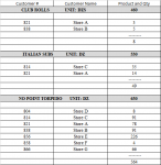
If you're willing to do a little prep to the input sheet, you can do it with either SUMIFS() or SUMPRODUCT(). The prep would involve this... put the product number on each row where there is an order (to the right of the quantity column). Secondly, if you use the SUMPRODUCT() solution, remove the pseudo underlines (---------). here's what I get:

Bakers Dozen.xlsx
	A	B	C	D	E	F	G	H	I	J	K	L	M	N
1	Customer #	Customer Name	Product and Qty
2	CLUB ROLLS	UNIT: DZS	460			SUMIFS()					SUMPRODUCT()
3							460	530	630			460	530	630
4	821	Store A	3	460		Store A	3	14	78		Store A	3	14	78
5	838	Store B	5	460		Store B	5	-	91		Store B	5	-	91
6						Store C	-	35	91		Store C	-	35	91
7			8			Store D	-	-	8		Store D	-	-	8
8						Store E	-	-	226		Store E	-	-	226
9	ITALIAN SUBS	UNIT: DZ	530			Store F	-	-	4		Store F	-	-	4
10						Store G	-	-	66		Store G	-	-	66
11	814	Store C	35	530
12	821	Store A	14	530
13
14			49
15
16	NO POINT TORPEDO	UNIT: DZ	630
17
18	804	Store D	8	630
19	814	Store C	91	630
20	821	Store A	78	630
21	88	Store B	91	630
22	856	Store E	226	630
23	858	Store F	4	630
24	866	Store G	66	630
25
26			564
Sheet1

Cell Formulas
Range	Formula
G4:I10	G4	=SUMIFS($C$4:$C$30,$B$4:$B$30,$F4,$D$4:$D$30,G$3)
L4:N10	L4	=SUMPRODUCT(($K4=$B$4:$B$30)*($D$4:$D$30=L$3)*($C$4:$C$30))
C7,C14	C7	=C4+C5
C26	C26	=SUM(C18:C24)

 

[DanteAmor]

Here another option with an array formula for you to consider:

Array formulas
Entered with Ctrl+Shift+Enter. If entered correctly, Excel will surround with curly braces {}.

Dante Amor.xlsm
	A	B	C	D	E	F	G	H
1	Customer #	Name	Product			460	530	630
2	CLUB ROLLS	UNIT: DZS	460		Store A	3	14	78
3					Store B	5		91
4	821	Store A	3		Store C		35	91
5	838	Store B	5
6
7	ITALLIAN SUBS	UNIT: DZS	530
8
9	814	Store C	35
10	821	Store A	14
11
12	NO POINT	UNIT: DZS	630
13
14	804	Store D	8
15	814	Store C	91
16	821	Store A	78
17	838	Store B	91
18	856	Store E	226
19	858	Store F	4
20	866	Store G	66
Sheet4

Cell Formulas
Range	Formula
F2:H4	F2	=IFERROR(VLOOKUP($E2,INDEX($B:$B,MATCH("UNIT*|"&F$1,LEFT($B$2:$B$200,4)&"|"&$C$2:$C$200,0)+1):INDEX($C:$C,IFERROR(MATCH("UNIT*|"&G$1,LEFT($B$2:$B$200,4)&"|"&$C$2:$C$200,0)-1,200)),2,0),"")
Press CTRL+SHIFT+ENTER to enter array formulas surrounded with curly braces.

 

[IvanYerk]

Terrific - arrays are my kryptonite! how would you modify the formula if using the customer # instead

 

[DanteAmor]

Try this:

Dante Amor.xlsm
	A	B	C	D	E	F	G	H
1	Customer #	Name	Product			460	530	630
2	CLUB ROLLS	UNIT: DZS	460		821	3	14	78
3					838	5		91
4	821	Store A	3		814		35	91
5	838	Store B	5
6
7	ITALLIAN SUBS	UNIT: DZS	530
8
9	814	Store C	35
10	821	Store A	14
11
12	NO POINT	UNIT: DZS	630
13
14	804	Store D	8
15	814	Store C	91
16	821	Store A	78
17	838	Store B	91
18	856	Store E	226
19	858	Store F	4
20	866	Store G	66
Sheet4

Cell Formulas
Range	Formula
F2:H4	F2	=IFERROR(VLOOKUP($E2,INDEX($A:$A,MATCH("UNIT*|"&F$1,LEFT($B$2:$B$200,4)&"|"&$C$2:$C$200,0)+1):INDEX($C:$C,IFERROR(MATCH("UNIT*|"&G$1,LEFT($B$2:$B$200,4)&"|"&$C$2:$C$200,0)-1,200)),3,0),"")
Press CTRL+SHIFT+ENTER to enter array formulas surrounded with curly braces.

 

[IvanYerk]

This is awesome, works perfectly and it's GREAT karma you both are putting out in the universe being so helpful on here. Many, many, many, thanks for your time!

So it pains me throw one more wrinkle in the mix - the file from the baker comes in with the category titled cells merged (I.e. A2/B2, A7/B7, A12/B12), so when the formula has the "UNIT*| part, I have to unmerge those cells and type UNIT in the B2, B7 and B12 cells to get it to work right.

I tried all night to try and fix it myself but couldn't quite get it right.

 

[DanteAmor]

It is a headache the merged cells, if you can work without it, you would be working better.

But, try this:

=IFERROR(VLOOKUP($E2,INDEX($A:$A,MATCH("*UNIT*|"&F$1,$A$2:$A$200&"|"&$C$2:$C$200,0)+1):INDEX($C:$C,IFERROR(MATCH("*UNIT*|"&G$1,$A$2:$A$200&"|"&$C$2:$C$200,0)-1,200)),3,0),"")

 

[IvanYerk]

Agree, but formula appears to be working - again, a thousand thanks - love learning new ways to use Excel!

 

[DanteAmor]

Glad we could help & thanks for the feedback