GrandCanyon
New Member
- Joined
- Mar 24, 2022
- Messages
- 1
- Office Version
- 365
- Platform
- Web
Hi all,
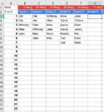
I'm taking over as organizer of a volunteer bicycle racing league series. The series is very straight forward. There are 22 weeks of racing (22 events). I want to record each riders result on a workbook 1st through (let's say) 50th, depending on how many people show up that week.
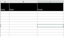
I'm then trying to get those results to update a separate workbook of season points standings which will assign the points, and calculate the running total of points attributed to that rider throughout the season. Points awarded are simple, they are the same as their finishing position, so this will be a lowest average score at the end of the season wins type of scenario.
To add a layer of complexity to this, the riders who show up will vary in attendance, some people will show up all 22 weeks, others will show up once so I don't want to create a separate roster tab. Instead, I'm attempting to have the series points standings page check the range of finishers and their respective positions by week and tabulate their average on the points standings page, and if the rider does not yet exist in the points standings, it should add them and assign their points. I've tried now many times, and have banging my head against the wall for a couple months now and the season begins in a few weeks. Might anyone be able to help?")
TL;DR I'm looking for a solution that will go through every cell in a range in one workbook (Race Results), check to see if it's value = anything in the other workbook (Series points standings) and, if true, add the value of that row (or finishing position, which is listed in column 1), if the value (the unique rider's name) is not found, add the value of that cell (the unique rider's name) to the standings list and add the value of that row (Finishing position, which is listed in column 1) next to, and correspondent to, the newly added value's (unique rider's name) row in column B. Then sort by ascending points average.
Might anyone know how to accomplish this?
I'm taking over as organizer of a volunteer bicycle racing league series. The series is very straight forward. There are 22 weeks of racing (22 events). I want to record each riders result on a workbook 1st through (let's say) 50th, depending on how many people show up that week.
I'm then trying to get those results to update a separate workbook of season points standings which will assign the points, and calculate the running total of points attributed to that rider throughout the season. Points awarded are simple, they are the same as their finishing position, so this will be a lowest average score at the end of the season wins type of scenario.
To add a layer of complexity to this, the riders who show up will vary in attendance, some people will show up all 22 weeks, others will show up once so I don't want to create a separate roster tab. Instead, I'm attempting to have the series points standings page check the range of finishers and their respective positions by week and tabulate their average on the points standings page, and if the rider does not yet exist in the points standings, it should add them and assign their points. I've tried now many times, and have banging my head against the wall for a couple months now and the season begins in a few weeks. Might anyone be able to help?
TL;DR I'm looking for a solution that will go through every cell in a range in one workbook (Race Results), check to see if it's value = anything in the other workbook (Series points standings) and, if true, add the value of that row (or finishing position, which is listed in column 1), if the value (the unique rider's name) is not found, add the value of that cell (the unique rider's name) to the standings list and add the value of that row (Finishing position, which is listed in column 1) next to, and correspondent to, the newly added value's (unique rider's name) row in column B. Then sort by ascending points average.
Might anyone know how to accomplish this?