Calculate average and max for specific dates

[latorta]

Hello,

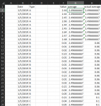
I am stuck and can't figure out how to obtain the max and average using the Value column for a large dataset (300K+) using what I think is two criteria (Date, Type) I want to get the average and max for each type based on the unique dates. The type of data repeats, e.i, A, B, C, but it corresponds to different dates. I want each date to have its own average and max based on the data type. Below you can see what I mean.

I tried the following for the average, IF(A2=A1,"",AVERAGEIF($A$2:$A$73,A2,$E$2:$E$73)), but It gives me the average for everything that has the same date, so I know it's wrong. The code below shows what I need using average and max.

Book2.xlsx
	A	B	C	D	E
1	Date	Type	Average	Max	Value
2	2019-01-01	A	2.496666667	2.66	2.44
3	2019-01-01	A	2.496666667	2.66	2.44
4	2019-01-01	A	2.496666667	2.66	2.45
5	2019-01-01	A	2.496666667	2.66	2.66
6	2019-01-01	A	2.496666667	2.66	2.44
7	2019-01-01	A	2.496666667	2.66	2.45
8	2019-01-01	A	2.496666667	2.66	2.64
9	2019-01-01	A	2.496666667	2.66	2.47
10	2019-01-01	A	2.496666667	2.66	2.48
11	2019-01-01	B	0.065333333	0.23	0.01
12	2019-01-01	B	0.065333333	0.23	0.01
13	2019-01-01	B	0.065333333	0.23	0.02
14	2019-01-01	B	0.065333333	0.23	0.23
15	2019-01-01	B	0.065333333	0.23	0.01
16	2019-01-01	B	0.065333333	0.23	0.02
17	2019-01-01	B	0.065333333	0.23	0.01
18	2019-01-01	B	0.065333333	0.23	0.01
19	2019-01-01	B	0.065333333	0.23	0.02
20	2019-01-01	B	0.065333333	0.23	0.23
21	2019-01-01	B	0.065333333	0.23	0.01
22	2019-01-01	B	0.065333333	0.23	0.02
23	2019-01-01	B	0.065333333	0.23	0.21
24	2019-01-01	B	0.065333333	0.23	0.04
25	2019-01-01	B	0.065333333	0.23	0.05
26	2019-01-01	C			0.21
27	2019-01-01	C			0.04
28	2019-01-01	C			0.05
29	2019-01-02	A	0.04	0.23	3.36
30	2019-01-02	A	0.04	0.23	3.36
31	2019-01-02	A	0.04	0.23	3.36
32	2019-01-02	A	0.04	0.23	3.5
33	2019-01-02	A	0.04	0.23	3.35
34	2019-01-02	A	0.04	0.23	3.36
35	2019-01-02	A	0.04	0.23	3.53
36	2019-01-02	A	0.04	0.23	3.35
37	2019-01-02	B			0.18
38	2019-01-02	B			0.05
39	2019-01-02	B			0.04
40	2019-01-02	B			0.05
41	2019-01-02	B			0.04
42	2019-01-02	B			0.04
43	2019-01-02	B			0.05
44	2019-01-02	B			5.7
45	2019-01-02	C			0.18
46	2019-01-02	C			0.05
47	2019-01-02	C			0.04
48	2019-01-02	C			0.05
49	2019-01-02	C			0.04
50	2019-01-02	C			0.04
51	2019-01-02	C			0.05
52	2019-01-02	C			5.7
53	2019-01-03	A			3.36
54	2019-01-03	A			3.35
55	2019-01-03	A			5.65
56	2019-01-03	A			5.66
57	2019-01-03	A			5.68
58	2019-01-03	A			5.68
59	2019-01-03	A			5.69
60	2019-01-03	A			3.94
61	2019-01-03	A			2.95
62	2019-01-03	A			0.02
63	2019-01-03	A			0.02
64	2019-01-03	B			3.94
65	2019-01-03	B			2.95
66	2019-01-03	B			0.02
67	2019-01-03	B			0.02
68	2019-01-03	B			0.02
69	2019-01-03	B			0.02
70	2019-01-03	B			3.36
71	2019-01-03	C			0.02
72	2019-01-03	C			0.02
73	2019-01-03	C			3.36
Sheet1

Cell Formulas
Range	Formula
C2:C10	C2	=AVERAGE($E$2:$E$10)
D2:D10	D2	=MAX($E$2:$E$10)
C11:C25	C11	=AVEDEV($E$11:$E$25)
D11:D25	D11	=MAX($E$11:$E$25)
C29:C36	C29	=AVERAGE($E$11:$E$18)
D29:D36	D29	=MAX($E$11:$E$18)

 

[AhoyNC]

Like this?

Book1
	A	B	C	D	E
1	Date	Type	Average	Max	Value
2	1/1/2019	A	2.496666667	2.66	2.44
3	1/1/2019	A	2.496666667	2.66	2.44
4	1/1/2019	A	2.496666667	2.66	2.45
5	1/1/2019	A	2.496666667	2.66	2.66
6	1/1/2019	A	2.496666667	2.66	2.44
7	1/1/2019	A	2.496666667	2.66	2.45
8	1/1/2019	A	2.496666667	2.66	2.64
9	1/1/2019	A	2.496666667	2.66	2.47
10	1/1/2019	A	2.496666667	2.66	2.48
11	1/1/2019	B	0.06	0.23	0.01
12	1/1/2019	B	0.06	0.23	0.01
13	1/1/2019	B	0.06	0.23	0.02
14	1/1/2019	B	0.06	0.23	0.23
15	1/1/2019	B	0.06	0.23	0.01
16	1/1/2019	B	0.06	0.23	0.02
17	1/1/2019	B	0.06	0.23	0.01
18	1/1/2019	B	0.06	0.23	0.01
19	1/1/2019	B	0.06	0.23	0.02
20	1/1/2019	B	0.06	0.23	0.23
21	1/1/2019	B	0.06	0.23	0.01
22	1/1/2019	B	0.06	0.23	0.02
23	1/1/2019	B	0.06	0.23	0.21
24	1/1/2019	B	0.06	0.23	0.04
25	1/1/2019	B	0.06	0.23	0.05
26	1/1/2019	C	0.1	0.21	0.21
27	1/1/2019	C	0.1	0.21	0.04
28	1/1/2019	C	0.1	0.21	0.05
29	1/2/2019	A	3.39625	3.53	3.36
30	1/2/2019	A	3.39625	3.53	3.36
31	1/2/2019	A	3.39625	3.53	3.36
32	1/2/2019	A	3.39625	3.53	3.5
33	1/2/2019	A	3.39625	3.53	3.35
34	1/2/2019	A	3.39625	3.53	3.36
35	1/2/2019	A	3.39625	3.53	3.53
36	1/2/2019	A	3.39625	3.53	3.35
37	1/2/2019	B	0.76875	5.7	0.18
38	1/2/2019	B	0.76875	5.7	0.05
39	1/2/2019	B	0.76875	5.7	0.04
40	1/2/2019	B	0.76875	5.7	0.05
41	1/2/2019	B	0.76875	5.7	0.04
42	1/2/2019	B	0.76875	5.7	0.04
43	1/2/2019	B	0.76875	5.7	0.05
44	1/2/2019	B	0.76875	5.7	5.7
45	1/2/2019	C	0.76875	5.7	0.18
46	1/2/2019	C	0.76875	5.7	0.05
47	1/2/2019	C	0.76875	5.7	0.04
48	1/2/2019	C	0.76875	5.7	0.05
49	1/2/2019	C	0.76875	5.7	0.04
50	1/2/2019	C	0.76875	5.7	0.04
51	1/2/2019	C	0.76875	5.7	0.05
52	1/2/2019	C	0.76875	5.7	5.7
53	1/3/2019	A	3.818181818	5.69	3.36
54	1/3/2019	A	3.818181818	5.69	3.35
55	1/3/2019	A	3.818181818	5.69	5.65
56	1/3/2019	A	3.818181818	5.69	5.66
57	1/3/2019	A	3.818181818	5.69	5.68
58	1/3/2019	A	3.818181818	5.69	5.68
59	1/3/2019	A	3.818181818	5.69	5.69
60	1/3/2019	A	3.818181818	5.69	3.94
61	1/3/2019	A	3.818181818	5.69	2.95
62	1/3/2019	A	3.818181818	5.69	0.02
63	1/3/2019	A	3.818181818	5.69	0.02
64	1/3/2019	B	1.475714286	3.94	3.94
65	1/3/2019	B	1.475714286	3.94	2.95
66	1/3/2019	B	1.475714286	3.94	0.02
67	1/3/2019	B	1.475714286	3.94	0.02
68	1/3/2019	B	1.475714286	3.94	0.02
69	1/3/2019	B	1.475714286	3.94	0.02
70	1/3/2019	B	1.475714286	3.94	3.36
71	1/3/2019	C	1.133333333	3.36	0.02
72	1/3/2019	C	1.133333333	3.36	0.02
73	1/3/2019	C	1.133333333	3.36	3.36
Sheet1

Cell Formulas
Range	Formula
C2:C73	C2	=AVERAGEIFS($E$2:$E$73,$A$2:$A$73,$A2,$B$2:$B$73,$B2)
D2:D73	D2	=MAXIFS($E$2:$E$73,$A$2:$A$73,$A2,$B$2:$B$73,$B2)

 

[latorta]

Like this?

Book1
	A	B	C	D	E
1	Date	Type	Average	Max	Value
2	1/1/2019	A	2.496666667	2.66	2.44
3	1/1/2019	A	2.496666667	2.66	2.44
4	1/1/2019	A	2.496666667	2.66	2.45
5	1/1/2019	A	2.496666667	2.66	2.66
6	1/1/2019	A	2.496666667	2.66	2.44
7	1/1/2019	A	2.496666667	2.66	2.45
8	1/1/2019	A	2.496666667	2.66	2.64
9	1/1/2019	A	2.496666667	2.66	2.47
10	1/1/2019	A	2.496666667	2.66	2.48
11	1/1/2019	B	0.06	0.23	0.01
12	1/1/2019	B	0.06	0.23	0.01
13	1/1/2019	B	0.06	0.23	0.02
14	1/1/2019	B	0.06	0.23	0.23
15	1/1/2019	B	0.06	0.23	0.01
16	1/1/2019	B	0.06	0.23	0.02
17	1/1/2019	B	0.06	0.23	0.01
18	1/1/2019	B	0.06	0.23	0.01
19	1/1/2019	B	0.06	0.23	0.02
20	1/1/2019	B	0.06	0.23	0.23
21	1/1/2019	B	0.06	0.23	0.01
22	1/1/2019	B	0.06	0.23	0.02
23	1/1/2019	B	0.06	0.23	0.21
24	1/1/2019	B	0.06	0.23	0.04
25	1/1/2019	B	0.06	0.23	0.05
26	1/1/2019	C	0.1	0.21	0.21
27	1/1/2019	C	0.1	0.21	0.04
28	1/1/2019	C	0.1	0.21	0.05
29	1/2/2019	A	3.39625	3.53	3.36
30	1/2/2019	A	3.39625	3.53	3.36
31	1/2/2019	A	3.39625	3.53	3.36
32	1/2/2019	A	3.39625	3.53	3.5
33	1/2/2019	A	3.39625	3.53	3.35
34	1/2/2019	A	3.39625	3.53	3.36
35	1/2/2019	A	3.39625	3.53	3.53
36	1/2/2019	A	3.39625	3.53	3.35
37	1/2/2019	B	0.76875	5.7	0.18
38	1/2/2019	B	0.76875	5.7	0.05
39	1/2/2019	B	0.76875	5.7	0.04
40	1/2/2019	B	0.76875	5.7	0.05
41	1/2/2019	B	0.76875	5.7	0.04
42	1/2/2019	B	0.76875	5.7	0.04
43	1/2/2019	B	0.76875	5.7	0.05
44	1/2/2019	B	0.76875	5.7	5.7
45	1/2/2019	C	0.76875	5.7	0.18
46	1/2/2019	C	0.76875	5.7	0.05
47	1/2/2019	C	0.76875	5.7	0.04
48	1/2/2019	C	0.76875	5.7	0.05
49	1/2/2019	C	0.76875	5.7	0.04
50	1/2/2019	C	0.76875	5.7	0.04
51	1/2/2019	C	0.76875	5.7	0.05
52	1/2/2019	C	0.76875	5.7	5.7
53	1/3/2019	A	3.818181818	5.69	3.36
54	1/3/2019	A	3.818181818	5.69	3.35
55	1/3/2019	A	3.818181818	5.69	5.65
56	1/3/2019	A	3.818181818	5.69	5.66
57	1/3/2019	A	3.818181818	5.69	5.68
58	1/3/2019	A	3.818181818	5.69	5.68
59	1/3/2019	A	3.818181818	5.69	5.69
60	1/3/2019	A	3.818181818	5.69	3.94
61	1/3/2019	A	3.818181818	5.69	2.95
62	1/3/2019	A	3.818181818	5.69	0.02
63	1/3/2019	A	3.818181818	5.69	0.02
64	1/3/2019	B	1.475714286	3.94	3.94
65	1/3/2019	B	1.475714286	3.94	2.95
66	1/3/2019	B	1.475714286	3.94	0.02
67	1/3/2019	B	1.475714286	3.94	0.02
68	1/3/2019	B	1.475714286	3.94	0.02
69	1/3/2019	B	1.475714286	3.94	0.02
70	1/3/2019	B	1.475714286	3.94	3.36
71	1/3/2019	C	1.133333333	3.36	0.02
72	1/3/2019	C	1.133333333	3.36	0.02
73	1/3/2019	C	1.133333333	3.36	3.36
Sheet1

Cell Formulas
Range	Formula
C2:C73	C2	=AVERAGEIFS($E$2:$E$73,$A$2:$A$73,$A2,$B$2:$B$73,$B2)
D2:D73	D2	=MAXIFS($E$2:$E$73,$A$2:$A$73,$A2,$B$2:$B$73,$B2)

Oh man, YES! Thank you so much. I really appreciate it. This was driving me mad.
I didn't realize I could use that function and set multiple criteria to reference and calculated what I needed.

 

[AhoyNC]

You're welcome. Thanks for the feedback and welcome to the forum.

 

[latorta]

You're welcome. Thanks for the feedback and welcome to the forum.

I have a follow-up question. Not sure if something is wrong with my 2016 Excel or I am doing something wrong. The formula you provided works, but for some reason, Excel copies the same value to every cell (90% of all cells). I tried to apply the formula manually to some of the sheets and get the same outcome as when I created a macro to apply this to a large number of sheets. I don't think it's updating (Formulas are set to automatically calculate). In the Average column I have the formula you've provided and to the right the value it's supposed to be using average. I notice that by re-saving the file and clicking I don't want it to be an xlsm It corrects itself, but this doesn't work on my dataset probably because it's so large. Currently, Excel is Calculating (8 threads) 44% Any idea?

Book3.xlsx
	A	B	C	D	E	F	G	H
1		Date	Type			Value	average	actual average
2		1/1/2019	A			2.44	2.496666667	2.496666667
3		1/1/2019	A			2.44	2.496666667	2.496666667
4		1/1/2019	A			2.45	2.496666667	2.496666667
5		1/1/2019	A			2.66	2.496666667	2.496666667
6		1/1/2019	A			2.44	2.496666667	2.496666667
7		1/1/2019	A			2.45	2.496666667	2.496666667
8		1/1/2019	A			2.64	2.496666667	2.496666667
9		1/1/2019	A			2.47	2.496666667	2.496666667
10		1/1/2019	A			2.48	2.496666667	2.496666667
11		1/1/2019	B			0.01	2.496666667	0.06
12		1/1/2019	B			0.01	2.496666667	0.06
13		1/1/2019	B			0.02	2.496666667	0.06
14		1/1/2019	B			0.23	2.496666667	0.06
15		1/1/2019	B			0.01	2.496666667	0.06
16		1/1/2019	B			0.02	2.496666667	0.06
17		1/1/2019	B			0.01	2.496666667	0.06
18		1/1/2019	B			0.01	2.496666667	0.06
19		1/1/2019	B			0.02	2.496666667	0.06
20		1/1/2019	B			0.23	2.496666667	0.06
21		1/1/2019	B			0.01	2.496666667	0.06
22		1/1/2019	B			0.02	2.496666667	0.06
23		1/1/2019	B			0.21	2.496666667	0.06
24		1/1/2019	B			0.04	2.496666667	0.06
25		1/1/2019	B			0.05	2.496666667	0.06
26		1/1/2019	C			0.21	2.496666667	0.1
27		1/1/2019	C			0.04	2.496666667	0.1
28		1/1/2019	C			0.05	2.496666667	0.1
29		1/2/2019	A			3.36	2.496666667
30		1/2/2019	A			3.36	2.496666667
31		1/2/2019	A			3.36	2.496666667
32		1/2/2019	A			3.5	2.496666667
33		1/2/2019	A			3.35	2.496666667
34		1/2/2019	A			3.36	2.496666667
35		1/2/2019	A			3.53	2.496666667
36		1/2/2019	A			3.35	2.496666667
37		1/2/2019	B			0.18	2.496666667
38		1/2/2019	B			0.05	2.496666667
39		1/2/2019	B			0.04	2.496666667
40		1/2/2019	B			0.05	2.496666667
41		1/2/2019	B			0.04	2.496666667
42		1/2/2019	B			0.04	2.496666667
43		1/2/2019	B			0.05	2.496666667
44		1/2/2019	B			5.7	2.496666667
45		1/2/2019	C			0.18	2.496666667
46		1/2/2019	C			0.05	2.496666667
47		1/2/2019	C			0.04	2.496666667
48		1/2/2019	C			0.05	2.496666667
49		1/2/2019	C			0.04	2.496666667
50		1/2/2019	C			0.04	2.496666667
51		1/2/2019	C			0.05	2.496666667
52		1/2/2019	C			5.7	2.496666667
53		1/3/2019	A			3.36	2.496666667
54		1/3/2019	A			3.35	2.496666667
55		1/3/2019	A			5.65	2.496666667
56		1/3/2019	A			5.66	2.496666667
57		1/3/2019	A			5.68	2.496666667
58		1/3/2019	A			5.68	2.496666667
59		1/3/2019	A			5.69	2.496666667
60		1/3/2019	A			3.94	2.496666667
61		1/3/2019	A			2.95	2.496666667
62		1/3/2019	A			0.02	2.496666667
63		1/3/2019	A			0.02	2.496666667
64		1/3/2019	B			3.94	2.496666667
65		1/3/2019	B			2.95	2.496666667
66		1/3/2019	B			0.02	2.496666667
67		1/3/2019	B			0.02	2.496666667
68		1/3/2019	B			0.02	2.496666667
69		1/3/2019	B			0.02	2.496666667
70		1/3/2019	B			3.36	2.496666667
71		1/3/2019	C			0.02	2.496666667
72		1/3/2019	C			0.02	2.496666667
73		1/3/2019	C			3.36	2.496666667
Sheet1

Cell Formulas
Range	Formula
H2:H10	H2	=AVERAGE(F2:F10)
H11:H25	H11	=AVERAGE($F$11:$F$25)
H26:H28	H26	=AVERAGE($F$26:$F$28)
G2:G73	G2	=AVERAGEIFS($F$2:$F$73,$B$2:$B$73,$B2,$C$2:$C$73,$C2)

 

[latorta]

It turns out I had to leave excel in a non-responding state after clicking calculate sheet in order to update every cell (2 Million calculations) to its correct value. It only took 44+ hours to update the value and to save.

 

[AhoyNC]

You might try using a pivot table. It's not going to be practical to use that many formulas. I'm not sure if there is a limit on how much data a pivot table can handle, but probably worth a try.
Maybe someone else can help with a VBA solution.