Calculate band on Hours/Time passed

[farhan11941234]

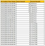
Please help me out to figure out a formula to calculate Date/Time Base Bins (See attached Image).Whenever The ID Creation(Column A) on Current Day and Time 3:00 PM to 6:00 PM, In Column C "> 3 to 6 PM" , Current Date and time between 6 to 7 PM in Column C result should be " > 6 to 7 PM", after 7:00 PM , in Column C should be "> 7:00 PM onwards.
when time > 14 Hours it should be >14 Hours and continue the this logic to >24 and >48 hours.
I would be very thankful to help me devolope the formula for this.

Sorry, for not using the XL2BB becuase of the admin Limitations.

Thanks

 

[farhan11941234]

I would be really helpful if the solution formula based on Column B where Hours are becuase in column A Date time is a text field in UK time formate dd/mm/yyyy
and its difficult for me to change it back to US format which often result errors since start date from 1 to 11 becomes month rather than days.

 

[jdellasala]

I hope you're willing to try Power Query. It is set up to handle complicated time calculations like this a LOT better than Excel!
Starting with this Table named Timesheet:

Book1
	A	B
1	Time Stamp	Now
2	12/14/22 12:12 AM	12/15/22 3:03 PM
3	12/13/22 3:33 PM	12/15/22 3:03 PM
4	12/14/22 7:56 AM	12/15/22 3:03 PM
5	12/13/22 6:08 PM	12/15/22 3:03 PM
6	12/13/22 6:59 PM	12/15/22 3:03 PM
7	12/13/22 9:38 AM	12/15/22 3:03 PM
8	12/13/22 1:48 AM	12/15/22 3:03 PM
9	12/14/22 3:27 AM	12/15/22 3:03 PM
10	12/13/22 5:23 PM	12/15/22 3:03 PM
11	12/14/22 4:48 AM	12/15/22 3:03 PM
12	12/13/22 5:37 PM	12/15/22 3:03 PM
13	12/13/22 2:25 PM	12/15/22 3:03 PM
14	12/14/22 11:16 PM	12/15/22 3:03 PM
15	12/13/22 12:14 PM	12/15/22 3:03 PM
16	12/14/22 11:20 AM	12/15/22 3:03 PM
17	12/14/22 5:22 AM	12/15/22 3:03 PM
18	12/14/22 1:56 PM	12/15/22 3:03 PM
19	12/13/22 11:26 AM	12/15/22 3:03 PM
20	12/14/22 7:58 AM	12/15/22 3:03 PM
21	12/14/22 10:31 PM	12/15/22 3:03 PM
Sheet1

Pulled the Table into Power Query,

let
    Source = Excel.CurrentWorkbook(){[Name="Timesheet"]}[Content],
    ChangedType = Table.TransformColumnTypes(Source,{{"Time Stamp", type datetime}, {"Now", type datetime}}),
    InsertedTimeSubtraction = Table.AddColumn(ChangedType, "Total Hours", each [Now] - [Time Stamp], type duration),
    CalculatedTotalHours = Table.TransformColumns(InsertedTimeSubtraction,{{"Total Hours", Duration.TotalHours, type number}}),
    RoundedOff = Table.TransformColumns(CalculatedTotalHours,{{"Total Hours", each Number.Round(_, 1), type number}})
in
    RoundedOff

and just a few easy steps gets the answer, resulting in this:

Book1
	D	E	F
1	Time Stamp	Now	Total Hours
2	12/14/2022 00:12	12/15/2022 15:03	38.8
3	12/13/2022 15:33	12/15/2022 15:03	47.5
4	12/14/2022 07:56	12/15/2022 15:03	31.1
5	12/13/2022 18:08	12/15/2022 15:03	44.9
6	12/13/2022 18:59	12/15/2022 15:03	44.1
7	12/13/2022 09:38	12/15/2022 15:03	53.4
8	12/13/2022 01:48	12/15/2022 15:03	61.2
9	12/14/2022 03:27	12/15/2022 15:03	35.6
10	12/13/2022 17:23	12/15/2022 15:03	45.7
11	12/14/2022 04:48	12/15/2022 15:03	34.2
12	12/13/2022 17:37	12/15/2022 15:03	45.4
13	12/13/2022 14:25	12/15/2022 15:03	48.6
14	12/14/2022 23:16	12/15/2022 15:03	15.8
15	12/13/2022 12:14	12/15/2022 15:03	50.8
16	12/14/2022 11:20	12/15/2022 15:03	27.7
17	12/14/2022 05:22	12/15/2022 15:03	33.7
18	12/14/2022 13:56	12/15/2022 15:03	25.1
19	12/13/2022 11:26	12/15/2022 15:03	51.6
20	12/14/2022 07:58	12/15/2022 15:03	31.1
21	12/14/2022 22:31	12/15/2022 15:03	16.5
Sheet1

I obviously didn't use your sample. I generated the Time Stamp column like this:

Book1
	L
1	Timestamp
2	12/14/22 2:59 PM
Sheet1

Cell Formulas
Range	Formula
L2:L21	L2	=RANDARRAY(20,,DATEVALUE("12/13/2022"),DATEVALUE("12/14/2022"),TRUE)+RANDARRAY(20,,0,1,FALSE)
Dynamic array formulas.

Once I had the Date and Time, I Copy/Paste Valued the column, added NOW() to generate the stop time (not in sample) and let Power Query do the rest.
To do this with Formulas is much more difficult. Give it a try!

 

[farhan11941234]

that was helpful but it did not solve my problem, becuause the Hours calculation was including when I get the Data from database.What I need is to create
a Column next to hours column Name Hours Bands.
The formula I used for calculation is pasted below , Now I like to Have if the ID Creation Date is current Date and ID Creation time is between 3:00PM to 06:00PM
In Hours Band Column Should be "> 3 to 6PM" and if creation time between 6 to 7 then "6 to 7 PM" and next is when ID creation time > 7 then ">7 PM Onward". This Band for current date only as when the hours exceeds > 14 then " > 14 Hours" , ">24 Hours", "> 48 Hours".
I hope that you understand what I am trying to acheive.


Hours in Column "B"
=IF(B2>48,">48 hours", IF(B2>18, ">18 hours, <48 hours", "<18 hours"))

 

[jdellasala]

Sorry I didn't understand that. What you need is an APROXIMATE Lookup. This may not be exactly what you need, but should show you how to do what you need:

Book2
	A	B	C	D	E	F
1	Time Stamp	Hours	Category		Time	Category
2	12/14/22 12:12 AM	38.8	Midnight to 3 AM		12:00 AM	Midnight to 3 AM
3	12/13/22 3:33 PM	47.5	Noon to 3 PM		3:00 AM	Midnight to 3 AM
4	12/14/22 7:56 AM	31.1	3 AM to 6 AM		6:00 AM	3 AM to 6 AM
5	12/13/22 6:08 PM	44.9	3 PM to 6 PM		9:00 AM	6 AM to 9 AM
6	12/13/22 6:59 PM	44.1	3 PM to 6 PM		12:00 PM	9 AM to Noon
7	12/13/22 9:38 AM	53.4	6 AM to 9 AM		3:00 PM	Noon to 3 PM
8	12/13/22 1:48 AM	61.2	Midnight to 3 AM		6:00 PM	3 PM to 6 PM
9	12/14/22 3:27 AM	35.6	Midnight to 3 AM		9:00 PM	6 PM to 9 PM
10	12/13/22 5:23 PM	45.7	Noon to 3 PM		11:59 PM	9 PM to Midnight
11	12/14/22 4:48 AM	34.2	Midnight to 3 AM
12	12/13/22 5:37 PM	45.4	Noon to 3 PM
13	12/13/22 2:25 PM	48.6	9 AM to Noon
14	12/14/22 11:16 PM	15.8	6 PM to 9 PM
15	12/13/22 12:14 PM	50.8	9 AM to Noon
16	12/14/22 11:20 AM	27.7	6 AM to 9 AM
17	12/14/22 5:22 AM	33.7	Midnight to 3 AM
18	12/14/22 1:56 PM	25.1	9 AM to Noon
19	12/13/22 11:26 AM	51.6	6 AM to 9 AM
20	12/14/22 7:58 AM	31.1	3 AM to 6 AM
21	12/14/22 10:31 PM	16.5	6 PM to 9 PM
Sheet1

Cell Formulas
Range	Formula
C2:C21	C2	=XLOOKUP(TIMEVALUE(TEXT([@[Time Stamp]],"h:mm AM/PM")),TimeCategories[Time],TimeCategories[Category],,-1)

The Category table shows how much of a pain Time can be!
Note that the Lookup Value in the XLOOKUP formula TIMEVALUE(TEXT([@[Time Stamp]],"h:mm AM/PM")) is what I needed because the values in the Time Stamp column were actual Date/Time values. You would need to adapt depending on what format your data comes in as. It does need to be in a numeric format though, so that you can do the approximate lookup.
The Approximate Value part of the XLOOKUP formula is the -1 fourth parameter [match_mode] part of the formula. What that means is that XLOOKUP will find the first value in the lookup_array that is as large as possible without being more than the lookup_value and return the corresponding return_array item.

Hope that gets you on the right track!

 

[Dave Patton]

Your requirements are not clear.
A concise example with expected results would help. N.B. You can post an extract with the forum's tool named XL2BB.
You can review the following which is a different spin based on post #5.

Time.xlsm
	A	B	C	D	E	F
1	Time Stamp	Hours			Time	Category
2	14-Dec-22 0:12	38.8		Midnight to 3 AM	0	Midnight to 3 AM
3	13-Dec-22 15:33	47.5		3 PM to 6 PM	03:00	3 AM to 6 AM
4	14-Dec-22 7:56	31.1		6 AM to 9 AM	06:00	6 AM to 9 AM
5	13-Dec-22 18:08	44.9		6 PM to 9 PM	09:00	9 AM to Noon
6	13-Dec-22 18:59	44.1		6 PM to 9 PM	12:00	Noon to 3 PM
7	13-Dec-22 9:38	53.4		9 AM to Noon	15:00	3 PM to 6 PM
8	13-Dec-22 1:48	61.2		Midnight to 3 AM	18:00	6 PM to 9 PM
9	14-Dec-22 3:27	35.6		3 AM to 6 AM	21:00	9 PM to Midnight
10	13-Dec-22 17:23	45.7		3 PM to 6 PM
11	14-Dec-22 4:48	34.2		3 AM to 6 AM
12	13-Dec-22 17:37	45.4		3 PM to 6 PM
13	13-Dec-22 14:25	48.6		Noon to 3 PM
14	14-Dec-22 23:16	15.8		9 PM to Midnight
15	13-Dec-22 12:14	50.8		Noon to 3 PM
16	14-Dec-22 11:20	27.7		9 AM to Noon
17	14-Dec-22 5:22	33.7		3 AM to 6 AM
18	14-Dec-22 13:56	25.1		Noon to 3 PM
19	13-Dec-22 11:26	51.6		9 AM to Noon
20	14-Dec-22 7:58	31.1		6 AM to 9 AM
21	14-Dec-22 22:31	16.5		9 PM to Midnight
10d

Cell Formulas
Range	Formula
D2:D21	D2	=XLOOKUP(MOD(A2,1),$E$2:$E$9,$F$2:$F$9,,-1)

 

[farhan11941234]

Sorry I didn't understand that. What you need is an APROXIMATE Lookup. This may not be exactly what you need, but should show you how to do what you need:

Book2
	A	B	C	D	E	F
1	Time Stamp	Hours	Category		Time	Category
2	12/14/22 12:12 AM	38.8	Midnight to 3 AM		12:00 AM	Midnight to 3 AM
3	12/13/22 3:33 PM	47.5	Noon to 3 PM		3:00 AM	Midnight to 3 AM
4	12/14/22 7:56 AM	31.1	3 AM to 6 AM		6:00 AM	3 AM to 6 AM
5	12/13/22 6:08 PM	44.9	3 PM to 6 PM		9:00 AM	6 AM to 9 AM
6	12/13/22 6:59 PM	44.1	3 PM to 6 PM		12:00 PM	9 AM to Noon
7	12/13/22 9:38 AM	53.4	6 AM to 9 AM		3:00 PM	Noon to 3 PM
8	12/13/22 1:48 AM	61.2	Midnight to 3 AM		6:00 PM	3 PM to 6 PM
9	12/14/22 3:27 AM	35.6	Midnight to 3 AM		9:00 PM	6 PM to 9 PM
10	12/13/22 5:23 PM	45.7	Noon to 3 PM		11:59 PM	9 PM to Midnight
11	12/14/22 4:48 AM	34.2	Midnight to 3 AM
12	12/13/22 5:37 PM	45.4	Noon to 3 PM
13	12/13/22 2:25 PM	48.6	9 AM to Noon
14	12/14/22 11:16 PM	15.8	6 PM to 9 PM
15	12/13/22 12:14 PM	50.8	9 AM to Noon
16	12/14/22 11:20 AM	27.7	6 AM to 9 AM
17	12/14/22 5:22 AM	33.7	Midnight to 3 AM
18	12/14/22 1:56 PM	25.1	9 AM to Noon
19	12/13/22 11:26 AM	51.6	6 AM to 9 AM
20	12/14/22 7:58 AM	31.1	3 AM to 6 AM
21	12/14/22 10:31 PM	16.5	6 PM to 9 PM
Sheet1

Cell Formulas
Range	Formula
C2:C21	C2	=XLOOKUP(TIMEVALUE(TEXT([@[Time Stamp]],"h:mm AM/PM")),TimeCategories[Time],TimeCategories[Category],,-1)

The Category table shows how much of a pain Time can be!
Note that the Lookup Value in the XLOOKUP formula TIMEVALUE(TEXT([@[Time Stamp]],"h:mm AM/PM")) is what I needed because the values in the Time Stamp column were actual Date/Time values. You would need to adapt depending on what format your data comes in as. It does need to be in a numeric format though, so that you can do the approximate lookup.
The Approximate Value part of the XLOOKUP formula is the -1 fourth parameter [match_mode] part of the formula. What that means is that XLOOKUP will find the first value in the lookup_array that is as large as possible without being more than the lookup_value and return the corresponding return_array item.

Hope that gets you on the right track!

Thanks you so much for your time, With your help I am able to get the desired result. I also used used a macro for date conversion.

Formula = =IF(AND(DAY(A2)=DAY(TODAY()),B2<14),XLOOKUP(TIMEVALUE(TEXT(TIME(HOUR(A2),MINUTE(A2), SECOND(A2)),"h:mm AM/PM")),$C$2:$C$23,$D$2:$D$23,,-1),IF(B2>72,">72 Hours",IF(B2>48,">48 Hours",IF(B2>36,">36 Hours",IF(B2>24,">24 Hours",IF(B2>14,">14 Hours","<14 Hours"))))))

 

[Dave Patton]

Are the brackets that you are using correct? What should show for 3:27?
You could use a lookup for the hours part.

Time.xlsm
	H	I	J	K	L
1				Hours	Text
2		or	or	0	<= 14 Hours
3	>36 Hours	> 36 Hours	> 36 Hours	14.001	> 14 Hours
4				24.001	> 24 Hours
5				36.001	> 36 Hours
6				72.001	> 72 Hours
10d

Cell Formulas
Range	Formula
H3	H3	=IF(B2>72,">72 Hours",IF(B2>48,">48 Hours",IF(B2>36,">36 Hours",IF(B2>24,">24 Hours",IF(B2>14,">14 Hours","<14 Hours")))))
I3	I3	=LOOKUP(B2,K2:L6)
J3	J3	=LOOKUP(B2,aL)

J3 Names the lookup information.

 

[jdellasala]

Your requirements are not clear.
A concise example with expected results would help. N.B. You can post an extract with the forum's tool named XL2BB.
You can review the following which is a different spin based on post #5.

Time.xlsm
	A	B	C	D	E	F
1	Time Stamp	Hours			Time	Category
2	14-Dec-22 0:12	38.8		Midnight to 3 AM	0	Midnight to 3 AM
3	13-Dec-22 15:33	47.5		3 PM to 6 PM	03:00	3 AM to 6 AM
4	14-Dec-22 7:56	31.1		6 AM to 9 AM	06:00	6 AM to 9 AM
5	13-Dec-22 18:08	44.9		6 PM to 9 PM	09:00	9 AM to Noon
6	13-Dec-22 18:59	44.1		6 PM to 9 PM	12:00	Noon to 3 PM
7	13-Dec-22 9:38	53.4		9 AM to Noon	15:00	3 PM to 6 PM
8	13-Dec-22 1:48	61.2		Midnight to 3 AM	18:00	6 PM to 9 PM
9	14-Dec-22 3:27	35.6		3 AM to 6 AM	21:00	9 PM to Midnight
10	13-Dec-22 17:23	45.7		3 PM to 6 PM
11	14-Dec-22 4:48	34.2		3 AM to 6 AM
12	13-Dec-22 17:37	45.4		3 PM to 6 PM
13	13-Dec-22 14:25	48.6		Noon to 3 PM
14	14-Dec-22 23:16	15.8		9 PM to Midnight
15	13-Dec-22 12:14	50.8		Noon to 3 PM
16	14-Dec-22 11:20	27.7		9 AM to Noon
17	14-Dec-22 5:22	33.7		3 AM to 6 AM
18	14-Dec-22 13:56	25.1		Noon to 3 PM
19	13-Dec-22 11:26	51.6		9 AM to Noon
20	14-Dec-22 7:58	31.1		6 AM to 9 AM
21	14-Dec-22 22:31	16.5		9 PM to Midnight
10d

Cell Formulas
Range	Formula
D2:D21	D2	=XLOOKUP(MOD(A2,1),$E$2:$E$9,$F$2:$F$9,,-1)

Really? That's the same exact thing except you didn't use a Table which not only does it make very clear what's going on, and expand/contract as needed with no change in formulas, but also prevents cell locking mistakes. There are few reasons to NOT use a full Excel Table instead of flat addresses.

 

[Dave Patton]

If you prefer, you can use a Table, Name the range of lookup information, or name the array of lookup information.

The Lookup information is not the same. Post #5 has the category "Midnight to 3 AM" twice.

Why do 3:27 and 5:22 AM show as Midnight to 3 AM?