Calculate Factors to Achieve Goal

[datasoup]

I'm having a challenge in resolving an algebraic problem using excel and would really appreciate some help.

Scenario:

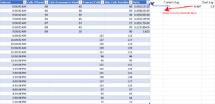
• Call center has goal of answering 80% of calls offered within X time
• Sum of calls currently answered at goal is 369
• Forecast remaining calls in day is 1854

Objective:

• How many calls need to be answered during the remaining intervals in order to reach the day goal?

 

[Eric W]

Welcome to the MrExcel forum!

Assuming you update your columns as shown in your example, try:

Book1
	A	B	C	D	E	F	G	H	I
1	Interval	Calls Offered	Calls Answered at Goal	Forecast Calls	Max Calls Possible	Ratio	# of calls needed	Current Avg	Goal Avg
2	6:00:00 AM	66	43		66	0.651515		0.647368	0.8
3	6:30:00 AM	85	56		85	0.658824
4	7:00:00 AM	90	59		90	0.655556			Remaining avg needed
5	7:30:00 AM	93	61		93	0.655914			0.846926
6	8:00:00 AM	87	57		87	0.655172
7	8:30:00 AM	69	43		69	0.623188
8	9:00:00 AM	80	50		80	0.625
9	9:30:00 AM			113	113		95.7
10	10:00:00 AM			117	117		99.1
11	10:30:00 AM			133	133		112.6
12	11:00:00 AM			139	139		117.7
13	11:30:00 AM			111	111		94.0
14	12:00:00 PM			96	96		81.3
15	12:30:00 PM			95	95		80.5
16	1:00:00 PM			101	101		85.5
17	1:30:00 PM			115	115		97.4
18	2:00:00 PM			131	131		110.9
19	2:30:00 PM			136	136		115.2
20	3:00:00 PM			127	127		107.6
21	3:30:00 PM			115	115		97.4
22	4:00:00 PM			87	87		73.7
23	4:30:00 PM			83	83		70.3
24	5:00:00 PM			84	84		71.1
25	5:30:00 PM			71	71		60.1
Sheet1

Cell Formulas
Range	Formula
F2:F25	F2	=IFERROR(C2/B2,"")
G2:G25	G2	=IF(F2<>"","",MAX(0,E2*$I$5))
H2	H2	=SUM(C2:C25)/SUM(B2:B25)
I5	I5	=(I2*SUM(E2:E25)-SUM(C2:C25))/(SUM(E2:E25)-SUM(B2:B25))

 

[datasoup]

Welcome to the MrExcel forum!

Assuming you update your columns as shown in your example, try:

Book1
	A	B	C	D	E	F	G	H	I
1	Interval	Calls Offered	Calls Answered at Goal	Forecast Calls	Max Calls Possible	Ratio	# of calls needed	Current Avg	Goal Avg
2	6:00:00 AM	66	43		66	0.651515		0.647368	0.8
3	6:30:00 AM	85	56		85	0.658824
4	7:00:00 AM	90	59		90	0.655556			Remaining avg needed
5	7:30:00 AM	93	61		93	0.655914			0.846926
6	8:00:00 AM	87	57		87	0.655172
7	8:30:00 AM	69	43		69	0.623188
8	9:00:00 AM	80	50		80	0.625
9	9:30:00 AM			113	113		95.7
10	10:00:00 AM			117	117		99.1
11	10:30:00 AM			133	133		112.6
12	11:00:00 AM			139	139		117.7
13	11:30:00 AM			111	111		94.0
14	12:00:00 PM			96	96		81.3
15	12:30:00 PM			95	95		80.5
16	1:00:00 PM			101	101		85.5
17	1:30:00 PM			115	115		97.4
18	2:00:00 PM			131	131		110.9
19	2:30:00 PM			136	136		115.2
20	3:00:00 PM			127	127		107.6
21	3:30:00 PM			115	115		97.4
22	4:00:00 PM			87	87		73.7
23	4:30:00 PM			83	83		70.3
24	5:00:00 PM			84	84		71.1
25	5:30:00 PM			71	71		60.1
Sheet1

Cell Formulas
Range	Formula
F2:F25	F2	=IFERROR(C2/B2,"")
G2:G25	G2	=IF(F2<>"","",MAX(0,E2*$I$5))
H2	H2	=SUM(C2:C25)/SUM(B2:B25)
I5	I5	=(I2*SUM(E2:E25)-SUM(C2:C25))/(SUM(E2:E25)-SUM(B2:B25))

Thank you kindly for the quick answer!

 

[Eric W]

Happy to help! Thanks for the feedback.