Calculate Tenure with a Twist

[mminchev]

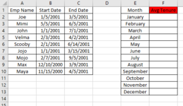
So I have two sheets. One sheet has my employee list with historic Start and End Dates. My other sheet is the summary of that list by Month. For example, lets say I have 10 Employees on my Employee sheet that all have Start and End dates, on my second sheet I have to summarize that info by Month and that includes showing Avg Tenure for all Employees that were at the company for that month.

Refer to the Image Below:

Please help I don't know why I cant figure this out, its one of those moments..... I really appreciate it!

 

[Toadstool]

Hi MMinchev,

Can you provide a worked example as it's not clear what you want.

• Is the Jan to Dec for a specific year?
• If so should tenure duration after that year/month be ignored?
• Have all staff left (i.e. no End Date will be blank).

 

[Sulprobil]

MrExcel_Calculate Tenure with a Twist.xlsx
	A	B	C	D	E	F
1	Emp Name	Start Date	End Date	Year	Month	Avg Tenure
2	Joe	05.01.2001	05.03.2001	2001	Januar	4,87096774
3	Mimi	05.05.2001	05.06.2001		Februar	7,71428571
4	John	01.01.2001	01.07.2001		März	5,93548387
5	Velma	03.02.2001	02.04.2001		April	3,23333333
6	Scooby	01.02.2001	14.06.2001		Mai	3,87096774
7	Jojo	01.01.2001	15.03.2001		Juni	2,63333333
8	Mojo	07.02.2001	05.09.2001		Juli	1,03225806
9	Max	10.12.2000	09.03.2001		August	1
10	Maya	15.11.2000	05.04.2001		September	0,16666667
11					Oktober	0
12					November	0
13					Dezember	0
14					Januar
Sheet1

Cell Formulas
Range	Formula
F2:F13	F2	=SUM(IF($B$2:$B$10<E3,IF($C$2:$C$10>=E2,IF($C$2:$C$10<E3-1,$C$2:$C$10,E3-1)-IF($B$2:$B$10>E2,$B$2:$B$10,E2)+1,0),0))/(E3-E2)
E2:E14	E2	=DATE($D$2,ROW()-1,1)
Press CTRL+SHIFT+ENTER to enter array formulas.

 

[mminchev]

MrExcel_Calculate Tenure with a Twist.xlsx
	A	B	C	D	E	F
1	Emp Name	Start Date	End Date	Year	Month	Avg Tenure
2	Joe	05.01.2001	05.03.2001	2001	Januar	4,87096774
3	Mimi	05.05.2001	05.06.2001		Februar	7,71428571
4	John	01.01.2001	01.07.2001		März	5,93548387
5	Velma	03.02.2001	02.04.2001		April	3,23333333
6	Scooby	01.02.2001	14.06.2001		Mai	3,87096774
7	Jojo	01.01.2001	15.03.2001		Juni	2,63333333
8	Mojo	07.02.2001	05.09.2001		Juli	1,03225806
9	Max	10.12.2000	09.03.2001		August	1
10	Maya	15.11.2000	05.04.2001		September	0,16666667
11					Oktober	0
12					November	0
13					Dezember	0
14					Januar
Sheet1

Cell Formulas
Range	Formula
F2:F13	F2	=SUM(IF($B$2:$B$10<E3,IF($C$2:$C$10>=E2,IF($C$2:$C$10<E3-1,$C$2:$C$10,E3-1)-IF($B$2:$B$10>E2,$B$2:$B$10,E2)+1,0),0))/(E3-E2)
E2:E14	E2	=DATE($D$2,ROW()-1,1)
Press CTRL+SHIFT+ENTER to enter array formulas.

Hi Sulprobil,

I appreciate it, however is this calculating running Avg Tenure up until that month for all employees that were available up until that time, because I am not understanding the numbers. For example, for January you are showing 4.871 Avg Tenure, can you explain how many employees that Avg is looking at? Furthermore, wouldn't the Avg Tenure for January be 1.6? I am just confused and if you could walk me through it would be great! Thank you again so much for this work.

 

[Sulprobil]

Hello,
Mojo is the only employee who was there through all of August, so August tenure is 1.
Since Mojo was there only until 5-Sep, the September tenure is 5/30 = 0.166667.
In January you had Maja, Max, Jojo, and John throughout the whole month which makes 4. Since Joe was there only from 5-Jan onwards you can add only 1-4/31 = 0.87096774. Which totals to 4.87096774 for January.
Regards,
Bernd