Calculate UPS Time In Transit Based on Zip Code

[ngarnold]

I'm trying to construct a formula that will calculate time in transit for UPS. I have a sheet "Sheet1"with tab that has a column that displays the five digit zip code "zip", and I have another tab "Sheet2" in that spreadsheet with a column for "Ground" (days in transit) and "Dest. ZIP"

The destination zip codes on Sheet2 are given as the first three digits of the zip code and (sometimes) in ranges, i.e 150-153 would represent zip codes 15000 to 15399. These are not in order, ex: 407-409 = 3, 260-261 = 2, 036 = 4

The columns on Sheet2 look like this (for example):

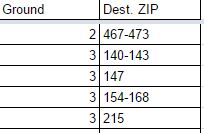
I want to make a formula that queries the cell "zip" on Sheet1, and returns a value "Ground" from Sheet2.

So if the zip code on Sheet1 in cell A2 is 46777, the formula would display 2 for the number of days in transit. If the zip code in Sheet1 A3 were 21525, the formula would display 3, if the zip is 14200 in Sheet1 A4 then 3...

Not sure if leading zeros on zip codes will cause an error? Presently those cells are set to display as plain text.

You can get the zone chart from UPS website here: https://www.ups.com/content/us/en/s...r+Shipping+Within+the+U.S.+and+to+Puerto+Rico

 

[DRSteele]

I hope I understood your objective.

The Dest_ZIP characters in column B are text and must be entered so (for example, the 215 is actually entered as '215); they also must be either 3 characters long or 7 characters long. The look-up values in column D are numbers and must be entered so.

Try this formula which relies on an array operation:

	A	B	C	D	E
1	Ground	Dest_ZIP		look-up	Ground
2	2	464-473		46777	2
3	3	140-143		21525	3
4	3	147		14200	3
5	3	154-168		3625	4
6	3	215
7	3	407-409
8	2	260-261
9	4	036

<tbody>
</tbody>

Sheet5​

Array Formulas Cell Formula E2 {=INDEX($A$2:$A$9,MATCH(TRUE,($D2>=100*LEFT($B$2:$B$9,3))=($D2<=IF(LEN($B$2:$B$9)=3,100*LEFT($B$2:$B$9,3)+99,RIGHT($B$2:$B$9,3)*100)),0))} <tbody> </tbody> Entered with Ctrl+Shift+Enter. If entered correctly, Excel will surround with curly braces {}. Note: Do not try and enter the {} manually yourself

<tbody>
</tbody>