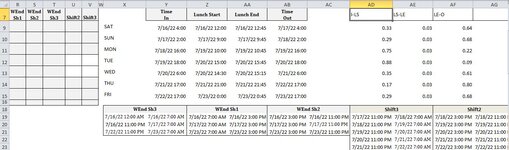
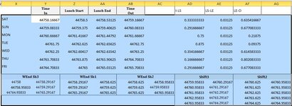
Here is an approach to consider. To write a formula-based solution, it is much more convenient to structure the supporting information as shown below. The time card data can be left as is, but a formula is used to transpose it so that Sat-Fri become column headings and the times in/out become row headings (see the transposed block in AR3:AY6). The shift descriptions originally occupied the range X18:AG23. For the sake of completeness, I added the weekday Shift1 descriptions (even though those have no differential...I'll explain why below). This extends the entire shift description range from X18:AI23. I don't think you need this, but it is arguably easier to read (for us), but not so convenient for referencing with formulas. I'm assuming these shift definitions are fairly rigid from week to week (e.g. weekend Shift 1 is always 7 AM to 3 PM). If that is true, then it is convenient to generate the shift table with a formula using only the starting point for the week (the Saturday date for the week is input in the blue cell AM11). Excel treats dates as numbers (as you've shown in your most recent post) and midnight of every day has an integer value (no decimal component). So the orange helper cells in AP13:AQ36 represent the number of fractional days to add to the starting point (i.e., midnight the date in AM11) to generate the start and end dates/times for each shift. I calculated these numbers by simply subtracting the shift start and end dates from the reference "0" point for the week (again, midnight the date in AM11) and saving the results as values only. So these orange cells are static and added to any new week start date in AM11 to generate the new shift table...that's what the pink cells in AN13:AO36 do, and the plain text description of the shift is given in the yellow cells in AM13:AM36.
Then the main computation block is found in AS13:AY36. A single formula is used here (pulled throughout the table) to look above at the in/out times for each day and compute the amount of time (in hours) that falls within the shift described on each row to the left. To do this, the basic formula for a single work "session" consists of four parts to establish how the start and end times of the work session compare to the start and end times of the shift. And since each day consists of two work sessions (before lunch and after lunch), the formula in each cell is repeated for the other work session. These are added together to obtain the total time worked on that day (for that column) during that shift (for that row). Then above the computation table, the total hours worked each day is shown (gray cells in AS10:AY10), which can be compared to the total hours worked, as computed directly from the time card data (the gray cells in AS7:AY7). This is why I felt it was important to include the weekday Shift1 (non differential) times...it allows for an error check to confirm that all of the worked time indicated by the timecard data has been apportioned among the various shifts. Then another sum is taken of only the hours worked during shifts that receive the differential (the red cells in AS9:AY9).
Finally, a SUMPRODUCT formula is used to sum the hours that match the day and shift shown in the summary table (green cells in R9:V15). One note...I've noticed before that adding and subtracting times can lead to some numeric precision issues (due to limitations with how Excel (and other programs) store numbers). To avoid having 8 hours appear as 7.999998611107 in the summary table, I've wrapped the SUMPRODUCT formula with a ROUND formula to round the results to 4 decimal places (which creates a rounding error less than 0.5 seconds).
You should be able to reconstruct this approach using the clipboard icon in the upper left of the mini sheet to copy it to your clipboard and
then navigate to an empty worksheet and paste into the same cell shown in the upper left of the posted mini sheet. Because of the size, I'm posting the sheet in two sections. To reconstitute the sheet, be sure to follow the italicized guidance in the last sentence.
I would consider deleting columns AK:AL as well as the shift definitions in X18:AI23 (they are not used anywhere and they are static...not changing when the week rolls over).
| Book3 |
|---|
|
|---|
| X | Y | Z | AA | AB | AC | AD | AE | AF | AG | AH | AI |
|---|
| 7 | | Time In | Lunch Start | Lunch End | Time Out | | | | | | | |
|---|
| 8 | | | | | | | | | | | | |
|---|
| 9 | SAT | 7/16/2022 4:00 | 7/16/2022 12:00 | 7/16/2022 12:45 | 7/17/2022 4:00 | | | | | | | |
|---|
| 10 | SUN | 7/17/2022 2:00 | 7/17/2022 9:00 | 7/17/2022 9:45 | 7/18/2022 2:00 | | | | | | | |
|---|
| 11 | MON | 7/18/2022 16:00 | 7/19/2022 10:00 | 7/19/2022 10:45 | 7/19/2022 16:00 | | | | | | | |
|---|
| 12 | TUE | 7/19/2022 18:00 | 7/20/2022 15:00 | 7/20/2022 15:45 | 7/20/2022 18:00 | | | | | | | |
|---|
| 13 | WED | 7/20/2022 6:00 | 7/20/2022 14:30 | 7/20/2022 15:15 | 7/21/2022 6:00 | | | | | | | |
|---|
| 14 | THU | 7/21/2022 17:00 | 7/21/2022 21:00 | 7/21/2022 21:45 | 7/22/2022 17:00 | | | | | | | |
|---|
| 15 | FRI | 7/22/2022 17:00 | 7/23/2022 0:00 | 7/23/2022 0:45 | 7/23/2022 17:00 | | | | | | | |
|---|
| 16 | | | | | | | | | | | | |
|---|
| 17 | | | | | | | | | | | | |
|---|
| 18 | WEnd Sh3 | | WEnd Sh1 | | WEnd Sh2 | | Shift3 | | Shift2 | | Shift1 (no differential) | |
|---|
| 19 | ####### | 7/16/2022 7:00 | 7/16/2022 7:00 | 7/16/2022 15:00 | 7/16/2022 15:00 | ###### | ###### | ###### | ###### | ###### | ###### | ###### |
|---|
| 20 | ####### | 7/17/2022 7:00 | 7/17/2022 7:00 | 7/17/2022 15:00 | 7/17/2022 15:00 | ###### | ###### | ###### | ###### | ###### | ###### | ###### |
|---|
| 21 | ####### | 7/23/2022 7:00 | 7/23/2022 7:00 | 7/23/2022 15:00 | 7/23/2022 15:00 | ###### | ###### | ###### | ###### | ###### | ###### | ###### |
|---|
| 22 | | | | | | | ###### | ###### | ###### | ###### | ###### | ###### |
|---|
| 23 | | | | | | | ###### | ###### | ###### | ###### | ###### | ###### |
|---|
|
|---|