Calculating the sum of a range or an area range where the start point can move

[Jules_Excel]

Hi folks,

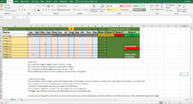
I've been tasked to create a spreadsheet which looks at the current month and sums the number of incidents in either a single range, or an area range, depending on a set of applied rules, based on a start point of the current month and looking back either 6 months, or 12 months, depending on which rule is being applied.

The data area will expand back 24 months, so as to cover the whole of the current year and of the previous year, but only a sufficient count within the scope of the rule-defined ranges should trigger the logic state to change. My example method (provided) broke on a 24 month history, as the logic kept triggering out of scope of the rules, so I really could use a better way of doing this.

I've bodged together a semi-working example covering just 1 year.

The rules are as follows:

#1: Count 2 or more under any singular category in any 6 months = Discuss
#2: Count 3 or more under any combined categories in any 6 months = Discuss
#3: Count 4 or more under any combined categories in any 12 months = Alert
#4: Any additional count over 4 in any category in any 12 months = Strong Alert


What I want to do to plot the area range (Please note: This is not how I've done it in the example sheet- this is the part I need help with):
- The start column position is given by a match based on the current month.
Note: This month value is currently set to a static value, but no need to worry about that.

- The starting row position is offset down by 2 to put the start point in the data area
- The end row range expands down 8 to the bottom of the data area
- The end column range looks left by 6, or 12, depending on the rule being applied
- The trigger logic is determined by each rule, depending on the sum in the defined area/range

Feel free to scrap my method entirely! - I'm really looking for a better, slicker example method of how to achieve this.

Thanks in advance!

 

[KRice]

Welcome to the board! Could you say a little more about the scope of this system, please? Your example shows one person and eight categories. Approximately how many people would be tracked with this system? And are the categories and number of categories the same for each person?

 

[Jules_Excel]

Thank you!

Sure. In response to your questions:

- There would be roughly 60 people tracked. The intention is to simply copy/paste a complete instance of the working chart in its entirety, for each individual, going down the worksheet.
- The number of categories are the same for each individual.

I appreciate you taking the time to have a look. TY!

 

[KRice]

Thanks for the clarification. I have a working example to try out, and perhaps you can let me know a little more about the rule sets. In this example, there are three table areas.

1. The main display table that looks similar to the one you described in your first post.
2. An incident data table located below the main display table. This data table is the one where monthly updates are made to record the number of incidents per category for the individual. There are no formulas in the data table. I've set up this table in the range A17:I139 to cover 10 years of reporting.
3. A helper computation table located to the right of the main display table. This is where the number of incidents occurring in various 6-month or 12-month blocks are tabulated. Additionally, this helper computation table contains the rule sets for Rules 1, 2, 3, and 4.

In operation, the user inputs the Evaluation Date in the blue cell AC9. This date is used to determine begin and end dates for the two-year period that contains the Evaluation Date as month number 24. And the two-year calendar labels in the main display table update based on these begin and end dates. Then formulas in the main data table match the category name and Month-Year heading to pull the corresponding number of incidents from the incident data table. The helper computation table located to the far right sums the incidents according to the rule sets you've described, although some additional clarification is needed (more on this below). The final results of the four rules are shown in cells AE13:AF16...these results are pulled into the main display table in cells Z4:AC4. Since Rule 1 involves evaluations against singular categories, the detailed Rule 1 results are found in AE5:AF12 and then pulled into the main display table in cells Z5:Z12. Conditional formatting is then applied to the summary rule results in Z4:AC4 based on the text in those cells.

With regard to the rules, I am not clear on whether these rules apply to the full two-year history or only a portion of it. This version assumes that the rules apply to all contiguous 6-month or 12-month blocks within the 2-year period that ends with the month-year of the Evaluation Date. Let me know if this is not correct.

The preferred way to share working examples is using the XL2BB add-in. To copy my sheet to your workbook, click on the clipboard icon in the upper left at the intersection of the row/column headings and then go to a blank worksheet and pasted into the same cell shown in the upper left of the posted example (cell A1 in this case).

The main display table and helper computation table are shown here (pasted in cell A1).

MrExcel20210214.xlsx
	A	B	C	D	E	F	G	H	I	J	K	L	M	N	O	P	Q	R	S	T	U	V	W	X	Y	Z	AA	AB	AC	AD	AE	AF	AG	AH	AI	AJ	AK	AL	AM	AN	AO	AP	AQ	AR	AS	AT	AU	AV	AW	AX	AY	AZ
1	Month #	1	2	3	4	5	6	7	8	9	10	11	12	13	14	15	16	17	18	19	20	21	22	23	24						Begin	3/1/2019
2	Mo-Yr	M-19	A-19	M-19	J-19	J-19	A-19	S-19	O-19	N-19	D-19	J-20	F-20	M-20	A-20	M-20	J-20	J-20	A-20	S-20	O-20	N-20	D-20	J-21	F-21						End	2/28/2021
3	Name:																									Rule 1	Rule 2	Rule 3	Rule 4
4	Joe Bloggs																									Discuss	Discuss	Alert	Strong Alert			6-mo blocks -->	1	2	3	4	5	6	7	8	9	10	11	12	13	14	15	16	17	18	19	Rule description
5	Category 1	1	0	0	0	0	0	0	0	0	0	0	0	0	0	0	0	0	0	0	0	1	2	3	0	Discuss					Rule 1	Discuss	1	0	0	0	0	0	0	0	0	0	0	0	0	0	0	1	3	6	6
6	Category 2	0	0	1	0	0	0	0	0	0	0	0	1	0	0	0	0	0	0	0	0	0	0	0	0						Rule 1		1	1	1	0	0	0	1	1	1	1	1	1	0	0	0	0	0	0	0
7	Category 3	0	0	0	0	0	0	0	2	0	0	0	0	0	0	0	0	0	1	0	0	0	0	0	0	Discuss					Rule 1	Discuss	0	0	2	2	2	2	2	2	0	0	0	0	1	1	1	1	1	1	0
8	Category 4	0	0	0	0	0	1	0	0	0	0	0	0	0	0	1	0	0	0	0	0	0	0	0	0				Eval Date		Rule 1		1	1	1	1	1	1	0	0	0	1	1	1	1	1	1	0	0	0	0
9	Category 5	0	0	0	0	0	0	0	0	0	0	2	0	0	0	0	0	2	0	0	0	0	0	0	0	Discuss			2/13/2021		Rule 1	Discuss	0	0	0	0	0	2	2	2	2	2	2	2	2	2	2	2	2	0	0
10	Category 6	0	0	0	0	0	0	1	0	0	0	0	0	0	0	0	0	0	0	1	0	0	0	0	0						Rule 1		0	1	1	1	1	1	1	0	0	0	0	0	0	1	1	1	1	1	1
11	Category 7	0	0	0	0	0	0	0	1	0	0	0	0	0	0	0	0	0	0	0	0	1	0	0	0						Rule 1		0	0	1	1	1	1	1	1	0	0	0	0	0	0	0	1	1	1	1
12	Category 8	0	0	0	0	0	0	0	0	2	0	0	0	0	0	0	0	0	0	0	0	0	0	0	2	Discuss					Rule 1	Discuss	0	0	0	2	2	2	2	2	2	0	0	0	0	0	0	0	0	0	2
13																															Rule 1	Discuss																				>=2 any 6 mo sing cat
14																															Rule 2	Discuss	3	3	6	7	7	9	9	8	5	4	4	4	4	5	5	6	8	9	10	>=3 any 6 mo comb cat
15																															Rule 3	Alert	12	11	11	11	11	13	13	13	10	10	12	13	14							>=4 any 12 mo comb cat
16																															Rule 4	Strong Alert	3	3	4	4	4	4	4	4	4	4	5	8	8							>4 any 12 mo sing cat
Jules_Excel

Cell Formulas
Range	Formula
B2:Y2	B2	=INDEX($A$20:$A$139,MATCH($AF$1,$A$20:$A$139,0)+COLUMNS($B2:B2)-1)
AF1	AF1	=DATE(YEAR($AC$9)-2,MONTH($AC$9)+1,1)
AF2	AF2	=EOMONTH($AC$9,0)
Z4	Z4	=AF13
AA4	AA4	=AF14
AB4	AB4	=AF15
AC4	AC4	=AF16
B5:Y12	B5	=INDEX($B$20:$I$139,MATCH(B$2,$A$20:$A$139,0),MATCH($A5,$B$19:$I$19,0))
Z5:Z12	Z5	=AF5
AG5:AY12	AG5	=SUM(OFFSET($A5,{0;1;2;3;4;5;6;7},{1,2,3,4,5,6,7,8,9,10,11,12,13,14,15,16,17,18,19},1,6))
AF5:AF12	AF5	=IF(COUNTIF(AG5:AY5,">="&2),"Discuss","")
AF13	AF13	=IF(COUNTIF(AF5:AF12,"Discuss"),"Discuss","Pass")
AF14	AF14	=IF(COUNTIF(AG14:AY14,">="&3),"Discuss","Pass")
AG14:AY14	AG14	=SUM(AG5:AG12)
AF15	AF15	=IF(COUNTIF(AG15:AS15,">="&4),"Alert","Pass")
AG15:AS15	AG15	=SUM(AG14,AM14)
AF16	AF16	=IF(COUNTIF(AG16:AS16,">"&4),"Strong Alert","Pass")
AG16:AS16	AG16	=SUM(MAX(AG5:AG12),MAX(AM5:AM12))
Press CTRL+SHIFT+ENTER to enter array formulas surrounded with curly braces.

Cells with Conditional Formatting
Cell	Condition		Cell Format	Stop If True
Z4:AC4	Cell Value	contains "Pass"	text	NO
Z4:AC4	Cell Value	contains "Discuss"	text	NO
Z4:AC4	Cell Value	contains "Strong Alert"	text	NO
Z4:AC4	Cell Value	contains "Alert"	text	NO

 

[KRice]

The incident data table should be created on the same sheet as the main display table. In this case, I created it beginning in cell A17. The headings found in B19:I19 should remain, as the matching formula in the main display table utilizes these labels. You can, however, hide the row if desired. For that matter, you can hide any of the rows that have already been filled out to effectively bring the current month closer to the top of the table.

MrExcel20210214.xlsx
	A	B	C	D	E	F	G	H	I
17	Incident Table:
18	Categories -->	1	2	3	4	5	6	7	8
19	keep labels -->	Category 1	Category 2	Category 3	Category 4	Category 5	Category 6	Category 7	Category 8
20	Jan-19
21	Feb-19
22	Mar-19	1
23	Apr-19
24	May-19		1
25	Jun-19
26	Jul-19
27	Aug-19				1
28	Sep-19						1
29	Oct-19			2				1
30	Nov-19								2
31	Dec-19
32	Jan-20					2
33	Feb-20		1
34	Mar-20
35	Apr-20
36	May-20				1
37	Jun-20
38	Jul-20					2
39	Aug-20			1
40	Sep-20						1
41	Oct-20
42	Nov-20	1						1
43	Dec-20	2
44	Jan-21	3
45	Feb-21								2
46	Mar-21
47	Apr-21							1
48	May-21
49	Jun-21						1
50	Jul-21		1
51	Aug-21					1
52	Sep-21
53	Oct-21
54	Nov-21			1
55	Dec-21				1
56	Jan-22
57	Feb-22
58	Mar-22
59	Apr-22
60	May-22
61	Jun-22
62	Jul-22
63	Aug-22
64	Sep-22
65	Oct-22
66	Nov-22
67	Dec-22
68	Jan-23
69	Feb-23
70	Mar-23
71	Apr-23
72	May-23
73	Jun-23
74	Jul-23
75	Aug-23
76	Sep-23
77	Oct-23
78	Nov-23
79	Dec-23
80	Jan-24
81	Feb-24
82	Mar-24
83	Apr-24
84	May-24
85	Jun-24
86	Jul-24
87	Aug-24
88	Sep-24
89	Oct-24
90	Nov-24
91	Dec-24
92	Jan-25
93	Feb-25
94	Mar-25
95	Apr-25
96	May-25
97	Jun-25
98	Jul-25
99	Aug-25
100	Sep-25
101	Oct-25
102	Nov-25
103	Dec-25
104	Jan-26
105	Feb-26
106	Mar-26
107	Apr-26
108	May-26
109	Jun-26
110	Jul-26
111	Aug-26
112	Sep-26
113	Oct-26
114	Nov-26
115	Dec-26
116	Jan-27
117	Feb-27
118	Mar-27
119	Apr-27
120	May-27
121	Jun-27
122	Jul-27
123	Aug-27
124	Sep-27
125	Oct-27
126	Nov-27
127	Dec-27
128	Jan-28
129	Feb-28
130	Mar-28
131	Apr-28
132	May-28
133	Jun-28
134	Jul-28
135	Aug-28
136	Sep-28
137	Oct-28
138	Nov-28
139	Dec-28
Jules_Excel

 

[KRice]

The helper computation table may be somewhat confusing. The table below might help explain what the formulas are doing. For a 24-month calendar, there are 19 sets of contiguous 6-month blocks and 13 sets of contiguous 12-month blocks, as shown in the two tables here. And if the 6-month blocks are processed first, one can derive the 12-month blocks by simply combining the correct two 6-month blocks, as summarized in cells A23:A35. The formulas essentially find these blocks and sum the incidents occurring within each.

MrExcel20210214.xlsx
	A	B	C	D	E	F	G	H	I	J	K	L	M	N	O	P	Q	R	S	T	U	V	W	X	Y	Z
2		6-mo blks \ mos	1	2	3	4	5	6	7	8	9	10	11	12	13	14	15	16	17	18	19	20	21	22	23	24
3		1	1	1	1	1	1	1
4		2		1	1	1	1	1	1
5		3			1	1	1	1	1	1
6		4				1	1	1	1	1	1
7		5					1	1	1	1	1	1
8		6						1	1	1	1	1	1
9		7							1	1	1	1	1	1
10		8								1	1	1	1	1	1
11		9									1	1	1	1	1	1
12		10										1	1	1	1	1	1
13		11											1	1	1	1	1	1
14		12												1	1	1	1	1	1
15		13													1	1	1	1	1	1
16		14														1	1	1	1	1	1
17		15															1	1	1	1	1	1
18		16																1	1	1	1	1	1
19		17																	1	1	1	1	1	1
20		18																		1	1	1	1	1	1
21		19																			1	1	1	1	1	1
22	6-mo blks	12-mo blks \ mos
23	1,7	1	1	1	1	1	1	1	1	1	1	1	1	1
24	2,8	2		1	1	1	1	1	1	1	1	1	1	1	1
25	3,9	3			1	1	1	1	1	1	1	1	1	1	1	1
26	4,10	4				1	1	1	1	1	1	1	1	1	1	1	1
27	5,11	5					1	1	1	1	1	1	1	1	1	1	1	1
28	6,12	6						1	1	1	1	1	1	1	1	1	1	1	1
29	7,13	7							1	1	1	1	1	1	1	1	1	1	1	1
30	8,14	8								1	1	1	1	1	1	1	1	1	1	1	1
31	9,15	9									1	1	1	1	1	1	1	1	1	1	1	1
32	10,16	10										1	1	1	1	1	1	1	1	1	1	1	1
33	11,17	11											1	1	1	1	1	1	1	1	1	1	1	1
34	12,18	12												1	1	1	1	1	1	1	1	1	1	1	1
35	13,19	13													1	1	1	1	1	1	1	1	1	1	1	1
Jules_Excel_explanation

 

[Jules_Excel]

Hello again,

Firstly, my apologies for taking so long in relying: I've been extremely busy. Secondly, thank you for taking the time for such a comprehensive response! Very much appreciated.

After a lot of digging around, I've decided on a solution that I feel best compliments how the end-users will be able to practically utilise the worksheet on an ongoing basis, in conjunction with the required functionality: there's a significant need for copying and pasting for each individual being monitored, so the more compact the solution, the better.

Solution
So, the table layout covers two years of data. This is all that's required, as the scope of the test range is, at most, 12 months. So as long as the previous years data exists to catch any overflow from early in the current year from the last year (for the 12 month test criteria), we're good to go.

Today's Date is set from the system using the TODAY() function. The Month is derived thereof, using MONTH(AC12) where AC12 is the cell containing the current date.

So now we know where we in the time-line - important, as I want to look from 'Now', back either 6 or 12 months depending on the Rule in question. To reference this, I've used the cells in row 2, starting on column N, with individual IF statements in each cell to place a numerical value that corresponds to the month; so 1 for Jan, 2 for Feb, and so on. So now each month knows its numerical position and I'll use this position as a start-point to calculate back the Rule-applicable 6 or 12 months range.

RULE #1:
Rule #1 is looking for an number of incidents greater than or equal to 2 in a single category

The matching for the Rule 1 single row ranges is achieved by:

=IF(SUM(OFFSET(N4,1,MATCH($AC$9,$N$2:$Y$2)-1,1,-6))>=2,1,0)

* The OFFSET references N4, which gives us an arbitrarily chosen starting position near the start of the data table.
The subsequent '1' indicates the row in which to look, with respect to the starting position mentioned above, in this case 'down 1 row', placing us in the left-uppermost row of the data table.
* The MATCH references the active month cell (currently populated with a '2' from the IF statement mentioned earlier. So now between those row and column coordinates, we've zeroed in on 'which row to look at' starting from which month.
* The -6 defines the 'previous 6 months from where we are currently'.
* And the SUM totals that row, and the IF looks for totals greater than or equal to 2.

Each of the helper cells directly under the Rule 1 column has a 0 or a 1 generated in it by the IF part of the statement, if the data row contains values equal to or greater than 2 in SUM.

The Rule 1 Pass/Fail reporting cell has an IF statement that looks for the occurrence of a 1 in any of the helper cells below, and changes state if a 1 is present, thereby neatly consolidating the reporting display to one cell.

RULE #2:
=IF(SUM(OFFSET(N4,1,MATCH($AC$9,$N$2:$Y$2)-1,8,-6))>=3,"Discuss","Pass")

Much the same method as described above, but the '8' defines an area range (as in: include all 8 rows, down from the column dated start position), as Rule 2 is looking for any incidents for any of the categories in a 6 month period, totalling equal to or greater than 3 occurrences.

RULE #3:
=IF(SUM(OFFSET(N4,1,MATCH(AC9,N2:Y2)-1,8,-12))>=4,"Alert","Pass")

The same as Rule #2, but with a 12 month area range now instead of 6.

RULE #4:
=IF(SUM(OFFSET(N4,1,MATCH(AC9,N2:Y2)-1,8,-12))>4,"Strong Alert","Pass")

... And so on for Rule #4, excepting that the IF condition has a higher trigger threshold.

Finally, at the end of the current year, the end-user will simply copy/paste this years data table values into last years table, and clear the data from the now, new current year, for each individual.


Thanks again for all your time and effort you've put into your example.

 

[KRice]

Thanks for the update. I'm glad you were able to arrive at a solution. Your explanation helped to clear up some questions I had. In post #1, you mentioned "looking back either 6 months, or 12 months" but later mentioned "in any 6 months" or "in any 12 months". I approached the problem as though you might need an assessment for the latter--in any 6 or 12 month block depending on the rule. It appears that you really want only one particular 6 or 12 month block...the ones ending in the current month...which would be the answer to a question I posed in post #4.

I am somewhat puzzled by your approach to Rule #4. In post #1, you mentioned "Any additional count over 4 in any category in any 12 months". My interpretation of "any category" was any singular category, while your formula is summing over all categories, just like Rule #3, but applying a slightly higher incident count threshold (>4 rather than >=4). I assumed, based on the post #1 description, that Rule #4 would look for the maximum value (not the sum) in each category within the 12-month block of interest.

 

[Jules_Excel]

Thanks for the update. I'm glad you were able to arrive at a solution. Your explanation helped to clear up some questions I had. In post #1, you mentioned "looking back either 6 months, or 12 months" but later mentioned "in any 6 months" or "in any 12 months". I approached the problem as though you might need an assessment for the latter--in any 6 or 12 month block depending on the rule. It appears that you really want only one particular 6 or 12 month block...the ones ending in the current month...which would be the answer to a question I posed in post #4.

I am somewhat puzzled by your approach to Rule #4. In post #1, you mentioned "Any additional count over 4 in any category in any 12 months". My interpretation of "any category" was any singular category, while your formula is summing over all categories, just like Rule #3, but applying a slightly higher incident count threshold (>4 rather than >=4). I assumed, based on the post #1 description, that Rule #4 would look for the maximum value (not the sum) in each category within the 12-month block of interest.

Yes, you are correct: I assert 'Any' as in 'All'. Semantically applicable, although now you mention it I see that 'All' might have been a clearer term.

I again use 'Any' in application to Rule #4 in the same context.

Glad we cleared that up!

Thanks again.

 

[KRice]

With regard to 6-month and 12-month blocks of time, post #1 uses the word "any" in all four rules. This implies that there are multiple time blocks, and that the rules apply to any of them. The problem statement is not clear about the fact that only one block of time is of interest---the one ending in the current month. It is now apparent that the intent was to convey that for any given input date, the assessment should consider only the past 6-month or 12-month block of time ending in the month of the input date, depending on the rule.

With regard to categories, the inconsistency remains. In post #1, Rule #1 refers to a "singular category", Rule #2 and Rule #3 both refer to "combined categories", and Rule #4 refers to "any category". The terms "singular" and "combined" are clear, but then "any category" is introduced in Rule #4. This means a single category, not multiple ones, as "category" is singular. Yet based on your solution, it appears that the intent was to convey that Rule #4 applies to combined categories, just like Rule #3.

The point is that the word "any" does not mean "all" and that the problem statement could have been clearer to avoid this confusion.