Can a formula replace the Offset's "Reference"?

[TrinityGal]

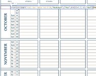
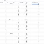
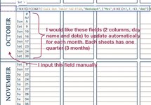
I have a question, what happens if you don't want to have a set reference, but you need to have that be taken from a callout table. For example, in a sheet I want to have the month on a cell, days in another column beside it with "ddd", only for Sat & Sun, and beside that column I want the date of such day. I want that information taken from a call out table in a separate sheet, where I have all the months from Jan-Feb, and where the dates and days are modified automatically when I update the year.

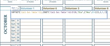
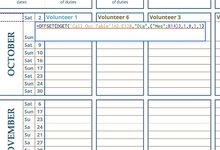
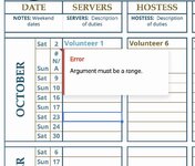
In my first sheet I want it to update the days and dates when I manually update the month, finding the month on my call out table with DGET, and selecting the first day and date respectively. That only works well with the first row. But for the other rows for the additional days and dates below the first row I want to use the OFFSET, but in the reference field I want it to find the corresponding month in the call out table based on what I manually enter in my first sheet for the month and based on that I want it to offset the results with the days and dates on the rows below the first one. Does that make sense? However, when I input the DGET formula in the reference section, it gives me an error saying "Argument myst be a range". Do you know what is happening and how I can fix it? Here is my formula:

=OFFSET(DGET('Call Out Table'!A2:E128,"Day",{"Month";B14}),1,0,1,1) I look forward to your reply! Thanks in advance!

 

[jasonb75]

it gives me an error saying "Argument myst be a range". Do you know what is happening and how I can fix it?

You can fix it by using a range. The offset reference must refer to a cell directly, not what is in the cell which is what the DGET function will be looking at.

In theory, you probably just need to refer to the top left cell of the table then use match for the row / column offsets. It would be easier to follow what you have with a visual representation of your sheet rather than just a description.

 

[TrinityGal]

Hi Jason.
Thanks for your reply!

I did do it by selecting one single cell on my call out table, more specifically the title of the column where I want the data from, but this does not work because when I make a new sheet for a new quarter of the year, and I update the months, the results are still selected from that top cell, giving me the results of the first three months.

Here is a link tot he document, which I published in Google sheets: https://docs.google.com/spreadsheet...JJATbCWGO543qV2q8ZufNLPVensDw/pub?output=xlsx

Does this help?

 

[jasonb75]

the results are still selected from that top cell,

That is not because offset is referring to a specific cell but because the row offset is fixed at 1. In principle you would use something on the format of
=OFFSET('Call Out Table'!$A$2,MATCH(something, somewhere, FALSE),0,1,1)
Where something and somewhere refer to a date to look for and a place to look for it, for example a specific date in a column of dates.
Given that you are only returning a single cell as the result, INDEX would by far be the preferable function to use.

I can't open your workbook due to security limitations, however there is a tool called XL2BB (<< link) that you can use to post your sample directly to the forum (only needs to be about 10 rows, not the whole thing).

 

[TrinityGal]

I've made a copy of the workbook with only two sheets, because I think you need to see the call-out table, or else the formulas would be broken, as they use data from that sheet.
Best I can do it upload images from that published version.

Does this help? It shows the formulas I am using and what I am trying to get, and where...

 

[TrinityGal]

Here are some notes about what I am after...

 

[jasonb75]

It's a bit of a formula unfriendly format but it should be possible. I don't think that I will be able to look at it today, hopefully another member will see your thread and provide a solution before I return.

 

[jasonb75]

See if this works, I've only done a very quick test so could have missed some errors.

Sample (3).xlsx
	B	C	D
14	OCTOBER	Sat	2
15		Sun	3
16		Sat	9
17		Sun	10
18		Sat	16
19		Sun	17
20		Sat	23
21		Sun	24
22		Sat	30
4TH QTR

Cell Formulas
Range	Formula
C14:C22	C14	=INDEX('Call Out Table'!$E:$E,MATCH(LOOKUP("zzz",$B$14:$B14),'Call Out Table'!$B:$B,0)+ROWS(C$14:C14)-MATCH("zzz",$B$14:$B14))
D14:D22	D14	=INDEX('Call Out Table'!$C:$C,MATCH(LOOKUP("zzz",$B$14:$B14),'Call Out Table'!$B:$B,0)+ROWS(C$14:C14)-MATCH("zzz",$B$14:$B14))

 

[Tetra201]

@TrinityGal: Wouldn't it be easier to have formulas calculating Saturdays and Sundays directly on your quarterly sheets -- instead of referring to the Call Out Table?

 

[johnnyL]

I can't open your workbook due to security limitations, however there is a tool called XL2BB (<< link) that you can use to post your sample directly to the forum (only needs to be about 10 rows, not the whole thing).

Here is the XL2BB Data ...

4TH QTR worksheet

Sample.xlsx
	A	B	C	D	E	F	G	H	I	J	K	L	M	N
1
2					OLA 2021 VOLUNTEER CALENDAR
3		DATE			SERVERS		HOSTESS		BUSSERS			COOKS		PRESENTER
4		NOTES: Weekend dates			SERVERS: Description of duties		HOSTESS: Description of duties		BUSSERS: Description of duties			COOKS: Description of duties		PRESENTER: Description of duties
13		Mes
14		OCTOBER	Sat	2	Volunteer 1		Volunteer 6		Volunteer 3			Volunteer 8		Presenter 1
15			Sun	#N/A
16			Sat	9
17			Sun	10
18			Sat	16
19			Sun	17
20			Sat	23
21			Sun	24
22			Sat	30
23
24		NOVEMBER	Sat	6
25			Sun	17
26			Su	23
27			Sa	24
28			Su	21
29			Sa	27
30			Su	28
31			Sa	34
32			Su	35
33
34		DECEMBER	Sa	4
35			Su	5
36			Sa	11
37			Su	12
38			Sa	18
39			Su	19
40			Sa	25
41			Su	26
4TH QTR

Call Out Table worksheet

Sample.xlsx
	A	B	C	D	E	F
1	2021
2	Month#	Mes	Dia	Weekday#	Day	# of Additional 7
3	1	January	2	7	Sat
4	1		3	1	Sun
5	1		9	7	Sat	1
6	1		10	1	Sun
7	1		16	7	Sat	2
8	1		17	1	Sun
9	1		23	7	Sat	3
10	1		24	1	Sun
11	1		30	7	Sat	4
12	1		31	1	Sun
13
14
15	2	February	6	7	Sat
16	2		7	1	Sun
17	2		13	7	Sat	1
18	2		14	1	Sun
19	2		20	7	Sat	2
20	2		21	1	Sun
21	2		27	7	Sat	3
22	2		28	1	Sun
23
24
25	3	March	6	7	Sat
26	3		7	1	Sun
27	3		13	7	Sat	1
28	3		14	1	Sun
29	3		20	7	Sat	2
30	3		21	1	Sun
31	3		27	7	Sat	3
32	3		28	1	Sun
33
34
35	4	April	3	7	Sat
36	4		4	1	Sun
37	4		10	7	Sat	1
38	4		11	1	Sun
39	4		17	7	Sat	2
40	4		18	1	Sun
41	4		24	7	Sat	3
42	4		25	1	Sun
43
44
45	5	May	1	7	Sat
46	5		2	1	Sun
47	5		8	7	Sat	1
48	5		9	1	Sun
49	5		15	7	Sat	2
50	5		16	1	Sun
51	5		22	7	Sat	3
52	5		23	1	Sun
53	5		29	7	Sat	4
54	5		30	1	Sun
55
56
57	6	June	5	7	Sat
58	6		6	1	Sun
59	6		12	7	Sat	1
60	6		13	1	Sun
61	6		19	7	Sat	2
62	6		20	1	Sun
63	6		26	7	Sat	3
64	6		27	1	Sun
65
66
67	7	July	3	7	Sat
68	7		4	1	Sun
69	7		10	7	Sat	1
70	7		11	1	Sun
71	7		17	7	Sat	2
72	7		18	1	Sun
73	7		24	7	Sat	3
74	7		25	1	Sun
75	7		31	7	Sat	4
76
77
78	8	August	1	1	Sun
79	8		7	7	Sat	1
80	8		8	1	Sun
81	8		14	7	Sat	2
82	8		15	1	Sun
83	8		21	7	Sat	3
84	8		22	1	Sun
85	8		28	7	Sat	4
86	8		29	1	Sun
87
88
89	9	September	4	7	Sat
90	9		5	1	Sun
91	9		11	7	Sat	1
92	9		12	1	Sun
93	9		18	7	Sat	2
94	9		19	1	Sun
95	9		25	7	Sat	3
96	9		26	1	Sun
97
98
99	10	October	2	7	Sat
100	10		3	1	Sun
101	10		9	7	Sat	1
102	10		10	1	Sun
103	10		16	7	Sat	2
104	10		17	1	Sun
105	10		23	7	Sat	3
106	10		24	1	Sun
107	10		30	7	Sat	4
108	10		31	1	Sun
109
110
111	11	November	6	7	Sat
112	11		7	1	Sun
113	11		13	7	Sat	1
114	11		14	1	Sun
115	11		20	7	Sat	2
116	11		21	1	Sun
117	11		27	7	Sat	3
118	11		28	1	Sun
119
120
121	12	December	4	7	Sat
122	12		5	1	Sun
123	12		11	7	Sat	1
124	12		12	1	Sun
125	12		18	7	Sat	2
126	12		19	1	Sun
127	12		25	7	Sat	3
128	12		26	1	Sun
Call Out Table

Cell Formulas
Range	Formula
B3,B121,B111,B99,B89,B78,B67,B57,B45,B35,B25,B15	B3	=TEXT(DATE($A$1,A3,1),"MMMM")
C3,C121,C111,C99,C89,C78,C67,C57,C45,C35,C25,C15	C3	=IF(WEEKDAY(DATE($A$1,A3,1))=1,1,8-WEEKDAY(DATE($A$1,A3,1)))
D3:D10	D3	=WEEKDAY(DATE($A$1,A$3,C3))
C122:C128,C112:C118,C100:C106,C90:C96,C79:C85,C68:C74,C58:C64,C46:C52,C36:C42,C26:C32,C16:C22,C4:C10	C4	=IF(D3=7,C3+1,C3+6)
C11,C65	C11	=IF(IF(D10=7,C10+1,C10+6)<=DAY(EOMONTH(DATE($A$1,A$3,1),0)),IF(D10=7,C10+1,C10+6),"")
D76,D43,D11:D12	D11	=IF(C11="","",WEEKDAY(DATE($A$1,A$3,C11)))
C12	C12	=IF(C11="","",IF(IF(D11=7,C11+1,C11+6)<=DAY(EOMONTH(DATE($A$1,A$3,1),0)),IF(D11=7,C11+1,C11+6),""))
F5,F69,F59,F47,F37,F27,F17	F5	=COUNTIF(D4:D5,D3)
F7,F61,F49,F39,F29,F19	F7	=COUNTIF(D4:D7,D3)
F9,F63,F51,F41,F31,F21	F9	=COUNTIF(D4:D9,D3)
F11,F53	F11	=COUNTIF(D4:D11,D3)
C14	C14	=IF(C23="","",IF(IF(D23=7,C23+1,C23+6)<=DAY(EOMONTH(DATE($A$1,A$15,1),0)),IF(D23=7,C23+1,C23+6),""))
D14,D23	D14	=IF(C14="","",WEEKDAY(DATE($A$1,A$15,C14)))
D15:D22	D15	=WEEKDAY(DATE($A$1,A$15,C15))
C23	C23	=IF(IF(D22=7,C22+1,C22+6)<=DAY(EOMONTH(DATE($A$1,A$15,1),0)),IF(D22=7,C22+1,C22+6),"")
A111:A118,A108,A57:A64,A54,A15:A22	A15	=A3+1
D25:D32	D25	=WEEKDAY(DATE($A$1,A$25,C25))
C33	C33	=IF(IF(D32=7,C32+1,C32+6)<=DAY(EOMONTH(DATE($A$1,A$25,1),0)),IF(D32=7,C32+1,C32+6),"")
D33	D33	=IF(C33="","",WEEKDAY(DATE($A$1,A$25,C33)))
A121:A128,A99:A106,A67:A74,A45:A52,A35:A42,A25:A32	A25	=A15+1
D35:D42	D35	=WEEKDAY(DATE($A$1,A$35,C35))
C43	C43	=IF(IF(D42=7,C42+1,C42+6)<=DAY(EOMONTH(DATE($A$1,A$35,1),0)),IF(D42=7,C42+1,C42+6),"")
D45:D52	D45	=WEEKDAY(DATE($A$1,A$45,C45))
C53	C53	=IF(IF(D52=7,C52+1,C52+6)<=DAY(EOMONTH(DATE($A$1,A$45,1),0)),IF(D52=7,C52+1,C52+6),"")
D53:D54	D53	=IF(C53="","",WEEKDAY(DATE($A$1,A$45,C53)))
C54	C54	=IF(C53="","",IF(IF(D53=7,C53+1,C53+6)<=DAY(EOMONTH(DATE($A$1,A$45,1),0)),IF(D53=7,C53+1,C53+6),""))
A53,A107,A89:A96,A78:A86,A75	A53	=A42+1
C56	C56	=IF(C65="","",IF(IF(D65=7,C65+1,C65+6)<=DAY(EOMONTH(DATE($A$1,A$3,1),0)),IF(D65=7,C65+1,C65+6),""))
D56,D65	D56	=IF(C56="","",WEEKDAY(DATE($A$1,A$57,C56)))
D57:D64	D57	=WEEKDAY(DATE($A$1,A$57,C57))
D67:D75	D67	=WEEKDAY(DATE($A$1,A$67,C67))
C75	C75	=IF(IF(D74=7,C74+1,C74+6)<=DAY(EOMONTH(DATE($A$1,A$67,1),0)),IF(D74=7,C74+1,C74+6),"")
C76	C76	=IF(C75="","",IF(IF(D75=7,C75+1,C75+6)<=DAY(EOMONTH(DATE($A$1,A$67,1),0)),IF(D75=7,C75+1,C75+6),""))
F71	F71	=COUNTIF(D69:D71,D67)
F73	F73	=COUNTIF(D69:D73,D67)
F75	F75	=COUNTIF(D69:D75,D67)
D78:D85	D78	=WEEKDAY(DATE($A$1,A$78,C78))
C86	C86	=IF(IF(D85=7,C85+1,C85+6)<=DAY(EOMONTH(DATE($A$1,A$78,1),0)),IF(D85=7,C85+1,C85+6),"")
D86:D87	D86	=IF(C86="","",WEEKDAY(DATE($A$1,A$78,C86)))
C87	C87	=IF(C86="","",IF(IF(D86=7,C86+1,C86+6)<=DAY(EOMONTH(DATE($A$1,A$78,1),0)),IF(D86=7,C86+1,C86+6),""))
F79	F79	=COUNTIF(D78:D79,D79)
F81	F81	=COUNTIF(D79:D81,D79)
F83	F83	=COUNTIF(D78:D83,D79)
F85	F85	=COUNTIF(D78:D85,D79)
D89:D96	D89	=WEEKDAY(DATE($A$1,A$89,C89))
C97	C97	=IF(IF(D96=7,C96+1,C96+6)<=DAY(EOMONTH(DATE($A$1,A$89,1),0)),IF(D96=7,C96+1,C96+6),"")
D97:D98	D97	=IF(C97="","",WEEKDAY(DATE($A$1,A$89,C97)))
C98	C98	=IF(C97="","",IF(IF(D97=7,C97+1,C97+6)<=DAY(EOMONTH(DATE($A$1,A$89,1),0)),IF(D97=7,C97+1,C97+6),""))
D99:D106	D99	=WEEKDAY(DATE($A$1,A$99,C99))
C107	C107	=IF(IF(D106=7,C106+1,C106+6)<=DAY(EOMONTH(DATE($A$1,A$99,1),0)),IF(D106=7,C106+1,C106+6),"")
D107:D108	D107	=IF(C107="","",WEEKDAY(DATE($A$1,A$99,C107)))
C108	C108	=IF(C107="","",IF(IF(D107=7,C107+1,C107+6)<=DAY(EOMONTH(DATE($A$1,A$99,1),0)),IF(D107=7,C107+1,C107+6),""))
F91,F123,F113,F101	F91	=COUNTIF(D89,D89)
F93,F125,F115,F103	F93	=COUNTIF(D89:D91,D89)
F95,F127,F117,F105	F95	=COUNTIF(D89:D93,D89)
F107	F107	=COUNTIF(D99:D105,D99)
D111:D118	D111	=WEEKDAY(DATE($A$1,A$111,C111))
C119	C119	=IF(IF(D118=7,C118+1,C118+6)<=DAY(EOMONTH(DATE($A$1,A$111,1),0)),IF(D118=7,C118+1,C118+6),"")
D119	D119	=IF(C119="","",WEEKDAY(DATE($A$1,A$111,C119)))
D121:D128	D121	=WEEKDAY(DATE($A$1,A$121,C121))