Can't understand why incorrect color fill being applied in VBA code

Ironman

Well-known Member
Joined
Jan 31, 2004
Messages
1,069
Office Version
  1. 365
Platform
  1. Windows
Hi

I was kindly given the below code many years ago. When the contents of a cell in Col H of sheet 'Training Log' are manually copied to a cell in Col E of sheet 'Analysis' and then the cell in Analysis is clicked, a hyperlink is created and the cell is filled the same shade as the cell in Col H of Training Log.

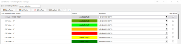
However, after I applied conditional formatting to Column H of Training Log, the colour copied is no longer correct and curiously is always the same colour (I also can't work out why it's that colour because none of the cells in either sheet are that colour).

Here's the code:
VBA Code:
Private Sub Worksheet_SelectionChange(ByVal Target As Range)
If Target.Column <> 5 Or Target.Cells.Count > 1 Then Exit Sub
If IsEmpty(Target) Then Exit Sub
Application.ScreenUpdating = False
Dim FindWhat$, FindWhere As Variant
FindWhat = Left(Target.Value, 255)

Set FindWhere = _
Sheets("Training Log").Columns(9).Find(What:=FindWhat, LookIn:=xlFormulas, lookat:=xlPart, MatchCase:=True)
If FindWhere Is Nothing Then Exit Sub

Dim iIndex%
iIndex = Sheets("Training Log").Cells(FindWhere.Row, 8).Interior.ColorIndex  '''''''''''this is the critical line
Target.Hyperlinks.Add _
Anchor:=Target, _
Address:="", _
SubAddress:="'Training Log'!I" & FindWhere.Row, _
TextToDisplay:="LOG ENTRY", _
ScreenTip:="Go to Training Log I" & FindWhere.Row
Target.Interior.ColorIndex = iIndex
With Target
.Font.Name = "Comic Sans MS"
.Font.Size = 7
.Font.Bold = True
.Font.Underline = xlUnderlineStyleSingle
Application.ScreenUpdating = True
End With

End Sub

I have another macro that does the same thing automatically i.e. copies the colour from the same column in Training Log, but to a different sheet as below, and it does it perfectly. I don't understand why the above doesn't work when I activate it by clicking the cell, but the below does when it's fully automated!
VBA Code:
If Target.Column = 8 And Target.Row = Range("A" & Rows.Count).End(xlUp).Row Then
Range("H" & Target.Row).Validation.Delete 'added 31.10.2021 - clears validation input info, no longer needed
    Lr1 = Target.Row
    If UCase(Trim(Left(Sheets("Training Log").Range("I" & Lr1).Value, 19))) = "INDOOR BIKE SESSION" Then
        Lr2 = Sheets("Indoor Bike").Range("A" & Rows.Count).End(xlUp).Row + 1
        Sheets("Indoor Bike").Range("F" & Lr2 & ":G" & Lr2).Value = Sheets("Training Log").Range("F" & Lr1 & ":G" & Lr1).Value  'ave heart rate
        Sheets("Indoor Bike").Range("I" & Lr2).Value = Sheets("Training Log").Range("H" & Lr1).Value  'session rating  '''''''''this is the critical line

I'd be very grateful for an amendment to the first macro so the cell in Col E of Analysis sheet is filled with the correct colour.

Thank you!
 
Last edited:

Excel Facts

Links? Where??
If Excel says you have links but you can't find them, go to Formulas, Name Manager. Look for old links to dead workbooks & delete.
If you have conditional formatting applied to the same range then that will be the cause.

The code is only changing the base fill colour of the cell, the same as if you changed it manually. If the conditions for a conditional formatting rule are met then that will override the base fill colour whether that is applied manually or by vba.

On the flip side, the code will not copy the colour applied by conditional formatting, only the base colour of the cell behind it. Reading your post a second time I think that this is more likely applicable to your scenario.
 
Upvote 0
Hi Jason, good to hear from you again, thanks for replying!

Sorry, I'm not at your level of understanding - why is the second macro working when it's pulling the data from the same conditionally formatted cell?

Just to clarify, conditional formatting is only applied in Col H of Training Log sheet.
 
Upvote 0
I did add a bit more to my last reply which I think you have likely missed.

Try saving a backup copy of your workbook for testing purposes, then delete the conditional formatting. Is the cell colour that you see after doing that the same as the one being copied?

With regard to the second piece of code, that is only copying values, not colours of any kind.
 
Upvote 0
Hi Jason, yes, the colour is correct once CF is removed.

The problem is I need to retain the CF in that column.

Is there any way round this so when I manually click the cell in Col E it copies the value (as per what you said above), so it will still work? To my way of thinking, there must be a 'common denominator' code that will allow it to work if the second code can run OK?
 
Upvote 0
The problem is I need to retain the CF in that column.
That means that the content of the cell is meeting the criteria for the cf to apply that colour.

Without having the full code and the data for testing I can only hazard a guess but I would say that the 2 different codes are not copying the same values and that if the second one was copying the same value as the first to a destination with the same cf rules then the same problem would occur.

At minimum, I would need to see the conditional formatting rule that is being applied, along with the values from the cells in order to diagnose the cause.
 
Upvote 0
Hi Jason, below are the CF rules and the values from the cells. They're a single letter in Wingdings format (to create a smiley) and the cell is in custom format ;;;"J"

Please let me know if you need any more info.

Thanks again.

Exercise Log Backup - Thursday 28 October 2021, 11.30 pm.xlsm
L
1Validation Col H
2J
3J
4J
5J
6K
7L
Training Log
 

Attachments

  • CF Col H.png
    CF Col H.png
    43.1 KB · Views: 19
Upvote 0
If you tick the Cond. formatting box on the XL2BB tab before clicking the Mini Sheet button then it includes the rules as part of the capture, you don't need to screen cap them separately.
Please let me know if you need any more info.
Which of the rules is being applied incorrectly and what is the value in the cell where it is being applied?
 
Upvote 0
Ah yes, sorry, I unchecked that a while back and forget to recheck it, thanks for reminding me.

All of the rules are being applied incorrectly, with the same color shade for all of them: #CCFFCC - as I mentioned, I have no idea where that colour comes from because I've never used that shade.

The values are either J, K or L.
 
Upvote 0
Have a look at link formatting, see if that is the cause.

From the information that you have provided so far, I can see no reason why it is doing what you say.

Can you upload the workbook to dropbox / onedrive and post a link to it here so that we can evaluate it? Without that, I don't think that identifying the cause is going to be possible.
 
Upvote 0

Forum statistics

Threads
1,214,643
Messages
6,120,702
Members
448,980
Latest member
CarlosWin

We've detected that you are using an adblocker.

We have a great community of people providing Excel help here, but the hosting costs are enormous. You can help keep this site running by allowing ads on MrExcel.com.
Allow Ads at MrExcel

Which adblocker are you using?

Disable AdBlock

Follow these easy steps to disable AdBlock

1)Click on the icon in the browser’s toolbar.
2)Click on the icon in the browser’s toolbar.
2)Click on the "Pause on this site" option.
Go back

Disable AdBlock Plus

Follow these easy steps to disable AdBlock Plus

1)Click on the icon in the browser’s toolbar.
2)Click on the toggle to disable it for "mrexcel.com".
Go back

Disable uBlock Origin

Follow these easy steps to disable uBlock Origin

1)Click on the icon in the browser’s toolbar.
2)Click on the "Power" button.
3)Click on the "Refresh" button.
Go back

Disable uBlock

Follow these easy steps to disable uBlock

1)Click on the icon in the browser’s toolbar.
2)Click on the "Power" button.
3)Click on the "Refresh" button.
Go back
Back
Top