Cell Completetion

[Kpjacques]

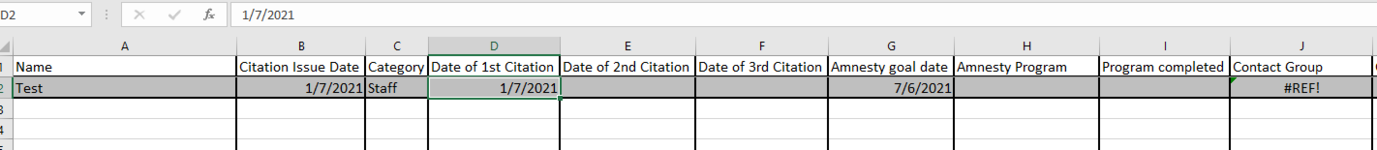
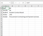
I am attempting to have one column fill with one of 5 responses based on what is typed in another column. In this case, my C column can have 1 of 5 values placed into it (Staff, Faculty, Student, Visitor, and Vendor), from there I want my J Column to have another word placed into it. I am not quite getting this to work for me. Any advice on how to get this to work?

 

[Joe4]

Welcome to the Board!

You should be able to do this by creating a lookup list (first column contains number, second the string to associate with each number).
Then you should be able use a simple VLOOKUP formula to return the looked up value when a number is entered in another cell.

See here for details and examples: MS Excel: How to use the VLOOKUP Function (WS)
If you run into issues, post your formula attempt and we should be able to help you fix it.

 

[Kpjacques]

=VLOOKUP(C2, Sheet1!A1:B5,10,FALSE)

Not sure what is going wrong here. C Column on the Log sheet is where I am entering the category, I want the J column on the log sheet to fill from a table on sheet 1.

 

[Joe4]

Your lookup range (second argument) should contain the column you want to include, i.e.
=VLOOKUP(C2, Sheet1!A1:J5,10,FALSE)
(how can you return the 10th column of a 2 column range?)

 

[Kpjacques]

I think I am misunderstood. The J Column is where the result is going not where the table ends. The table is A to B on Sheet one. The J column is on the Log sheet where the result must go after one of the values in the C column in the log sheet is typed (Staff, Student, etc...)

 

[Kpjacques]

Here are pictures of what I am talking about.

 

[Joe4]

Then it is the third argument of your formula that you must update:
=VLOOKUP(C2, Sheet1!A1:B5,2,FALSE)

The formula does not care what cell you are putting it in.
The second and third arguments work in tandem.

The second argument is your lookup range. The first column MUST be the column you are looking in, and the range MUST include the value you want to look up.
The third argument wants to know the index number of the lookup range where the value you want to return resides.

So, if it is a 2 column range, and you want to return the second column, you enter a 2 in the third argument.

 

[Kpjacques]

Thank you, now it is working. That is most helpful.

 

[Joe4]

You are welcome.
Glad I was able to help.

The VLOOKUP formula can seem a little tricky the first time you do it, but after understand how it works and you use it a few times, it begins to make more sense.