Chart range that skips non-numerical data points

labratto

New Member
Joined
Feb 9, 2021
Messages
7
Office Version
  1. 365
Platform
  1. Windows
Hi all,
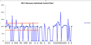
I am trying to make a chart that skips points that are not numbers. For the x-axis my values are coming from this named range formula (paintMSdatapointnumber) which shows the last specified number of values.
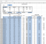
Excel Formula:
=OFFSET(' Paint'!$A$14,COUNT(' Paint'!$A:$A),0,-' Paint'!$X$11,1)
I thought with the count function it would skip the "" cells, but it appears that is not the case. The cells that appear blank have formulas in them that result in "" if there is no data entered into the parent cells.
The y values are the above names range with the column offset.
Excel Formula:
=OFFSET(paintMSdatapointnumber,0,4)

Can I make this work, or should I start over with a different strategy?
 

Attachments

  • Screenshot 2021-02-12 194358.png
    Screenshot 2021-02-12 194358.png
    38.1 KB · Views: 15
  • Screenshot 2021-02-12 194322.png
    Screenshot 2021-02-12 194322.png
    96.7 KB · Views: 14

Excel Facts

Format cells as time
Select range and press Ctrl+Shift+2 to format cells as time. (Shift 2 is the @ sign).
This is my first take on it. I usually create helper columns for the chart that filter the data I need. Column B provides a row number if the test is true. Columns E-G return the data based on row numbers

Book2 (version 1).xlsb
ABCDEFG
1NumbersRowY1Y2XvaluesY1 ValuesY2 Values
2112051205
322301023010
433401534015
544502045020
655602556025
7g0703068035
866803559040
9579040410045
104810045711050
117911050813060
12j012055914065
13810130601016075
1491114065   
15i015070   
16101216075   
Sheet2
Cell Formulas
RangeFormula
E2:E16E2=XLOOKUP(ROW()-1,$B$2:$B$16,$A$2:$A$16,"")
F2:F16F2=XLOOKUP(ROW()-1,$B$2:$B$16,$C$2:$C$16,"")
G2:G16G2=XLOOKUP(ROW()-1,$B$2:$B$16,$D$2:$D$16,"")
B2:B16B2=IF(ISNUMBER(A2),MAX($B$1:B1)+1,0)
 
Upvote 0
This is my first take on it. I usually create helper columns for the chart that filter the data I need. Column B provides a row number if the test is true. Columns E-G return the data based on row numbers

Book2 (version 1).xlsb
ABCDEFG
1NumbersRowY1Y2XvaluesY1 ValuesY2 Values
2112051205
322301023010
433401534015
544502045020
655602556025
7g0703068035
866803559040
9579040410045
104810045711050
117911050813060
12j012055914065
13810130601016075
1491114065   
15i015070   
16101216075   
Sheet2
Cell Formulas
RangeFormula
E2:E16E2=XLOOKUP(ROW()-1,$B$2:$B$16,$A$2:$A$16,"")
F2:F16F2=XLOOKUP(ROW()-1,$B$2:$B$16,$C$2:$C$16,"")
G2:G16G2=XLOOKUP(ROW()-1,$B$2:$B$16,$D$2:$D$16,"")
B2:B16B2=IF(ISNUMBER(A2),MAX($B$1:B1)+1,0)

I am attempting this solution, but my formula in for the second column (your B) always returns 0.
Excel Formula:
=IF(ISNUMBER('Paint Chart Data'!H15), MAX($A$3:A3)+1,0)
 
Upvote 0
I am attempting this solution, but my formula in for the second column (your B) always returns 0.
Excel Formula:
=IF(ISNUMBER('Paint Chart Data'!H15), MAX($A$3:A3)+1,0)
The numbers are not typed in, they are also a formula
 
Upvote 0
A formula resulting in a number will still test TRUE by ISNUMBER. Is your formula in column A? Is the cell number formatting set to a number and not text?
 
Upvote 0

Forum statistics

Threads
1,214,646
Messages
6,120,716
Members
448,985
Latest member
chocbudda

We've detected that you are using an adblocker.

We have a great community of people providing Excel help here, but the hosting costs are enormous. You can help keep this site running by allowing ads on MrExcel.com.
Allow Ads at MrExcel

Which adblocker are you using?

Disable AdBlock

Follow these easy steps to disable AdBlock

1)Click on the icon in the browser’s toolbar.
2)Click on the icon in the browser’s toolbar.
2)Click on the "Pause on this site" option.
Go back

Disable AdBlock Plus

Follow these easy steps to disable AdBlock Plus

1)Click on the icon in the browser’s toolbar.
2)Click on the toggle to disable it for "mrexcel.com".
Go back

Disable uBlock Origin

Follow these easy steps to disable uBlock Origin

1)Click on the icon in the browser’s toolbar.
2)Click on the "Power" button.
3)Click on the "Refresh" button.
Go back

Disable uBlock

Follow these easy steps to disable uBlock

1)Click on the icon in the browser’s toolbar.
2)Click on the "Power" button.
3)Click on the "Refresh" button.
Go back
Back
Top