Private Sub Frame1_Click()
End Sub
Private Sub Frame2_Click()
End Sub
Private Sub Label1_Click()
Dim i As Integer
r = Selection.Row
c = Selection.Column
Sheets("Folha2").Range("J10").Value = Sheets("Folha1").Cells(r, c - 1).Value
Sheets("Folha2").Range("F10").Value = Sheets("Folha1").Range("A" & r).Value
Sheets("Folha2").Range("D13").Value = Sheets("Folha1").Range("B" & r).Value
Sheets("Folha2").Range("I14").Value = Sheets("Folha1").Range("C" & r).Value
Sheets("Folha2").Range("D15").Value = Sheets("Folha1").Range("D" & r).Value
Sheets("Folha2").Range("D16").Value = Sheets("Folha1").Range("F" & r).Value
Sheets("Folha2").Range("D17").Value = Sheets("Folha1").Range("G" & r).Value
Sheets("Folha2").Range("D18").Value = Sheets("Folha1").Range("I" & r).Value
Sheets("Folha2").Range("K18").Value = Sheets("Folha1").Range("AD" & r).Value
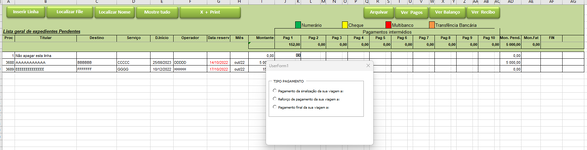
If UserForm1.OptionButton1.Value = True Then
Sheets("Folha2").Range("D14").Value = UserForm1.OptionButton1.Caption
End If
If UserForm1.OptionButton2.Value = True Then
Sheets("Folha2").Range("D14").Value = UserForm1.OptionButton2.Caption
End If
If UserForm1.OptionButton3.Value = True Then
Sheets("Folha2").Range("D14").Value = UserForm1.OptionButton3.Caption
End If
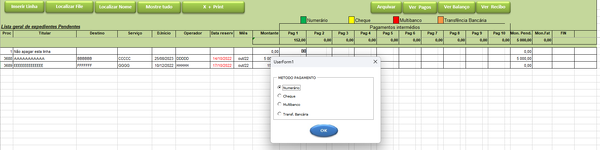
If UserForm1.OptionButton4.Value = True Then
Sheets("Folha2").Range("D11").Value = UserForm1.OptionButton4.Caption
End If
If UserForm1.OptionButton5.Value = True Then
Sheets("Folha2").Range("D11").Value = UserForm1.OptionButton5.Caption
End If
If UserForm1.OptionButton6.Value = True Then
Sheets("Folha2").Range("D11").Value = UserForm1.OptionButton6.Caption
End If
If UserForm1.OptionButton7.Value = True Then
Sheets("Folha2").Range("D11").Value = UserForm1.OptionButton7.Caption
End If
If UserForm1.OptionButton8.Value = True Then
Sheets("Folha2").Range("D11").Value = UserForm1.OptionButton8.Caption
End If
'r = Selection.Row
Unload Me
End Sub
Private Sub Label2_Click()
Unload Me
End Sub
Sub inserting_val(val As String, rr As Integer)
If Sheets("Folha1").Range(val & rr).Value = True Then
Sheets("Folha2").Range("J10").Value = Sheets("Folha1").Range(val & rr).Offset(0, -1).Value
Sheets("Folha1").CheckBoxes.Add(0, 0, 5, 5).Select
With Selection
.Value = True
.Display3DShading = False
.Caption = ""
End With
Selection.Cut
Sheets("Folha1").Range(val & rr).Select
Sheets("Folha1").Paste
Sheets("Folha1").Range("A1").Select
Sheets("Folha2").Range("F10").Value = Sheets("Folha1").Range("A" & rr).Value
Sheets("Folha2").Range("D13").Value = Sheets("Folha1").Range("B" & rr).Value
Sheets("Folha2").Range("I14").Value = Sheets("Folha1").Range("C" & rr).Value
Sheets("Folha2").Range("D14").Value = Sheets("Folha1").Range("D" & rr).Value
'Sheets("Folha2").Range("C10").Value = Sheets("Folha1").Range("D" & rr).Value
End If
End Sub
Private Sub optionButton1_Click()
UserForm1.Frame2.Visible = True
End Sub
Private Sub optionButton2_Click()
UserForm1.Frame2.Visible = True
End Sub
Private Sub optionButton3_Click()
UserForm1.Frame2.Visible = True
End Sub
Private Sub optionButton4_Click()
UserForm1.Label1.Visible = True
End Sub
Private Sub optionButton5_Click()
UserForm1.Label1.Visible = True
End Sub
Private Sub optionButton6_Click()
UserForm1.Label1.Visible = True
End Sub
Private Sub optionButton8_Click()
UserForm1.Label1.Visible = True
End Sub
Private Sub UserForm_Click()
End Sub
]
[CODE=vba]
Sub d_file()
UserForm2.Show
End Sub
Sub Caixadeverificação1_Click()
Dim celluletrouvee As Range
Dim ligne As Integer
Dim col As Integer
UserForm1.Show
'e = Range("A4").End(xlDown).Row
Sheets("Folha2").Select
End Sub
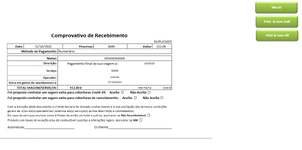
Sub CreerPDF(Nomme As String, CHQ As String, MB As String, TRF As String, zoom As Integer)
Dim date_file, save_path, save_file As String
Dim x As Long
date_test = Now()
date_file = CStr(Format(date_test, "ddmmyyyy"))
'save_root = "C:\Users\admin\Desktop\upwork"
'save_root = "C:\Users\Filipe\Desktop\upwork"
save_root = "\\PAULO-PC\Drive"
'save_root = "E:\"
save_path = save_root & "\" & CHQ
save_file = save_path & "\" & date_file & "+" & TRF & "+" & MB & "€.pdf"
RŽpertoireExiste (save_root)
RŽpertoireExiste (save_path)
'
With Sheets("Folha2").PageSetup
.Orientation = xlPortrait
.PaperSize = xlPaperA4
.FirstPageNumber = xlAutomatic
.Order = xlDownThenOver
.zoom = zoom
End With
With Sheets("Folha2")
.ExportAsFixedFormat _
Type:=xlTypePDF, _
Filename:=save_file, _
Quality:=xlQualityStandard, _
IncludeDocProperties:=True, _
IgnorePrintAreas:=False, _
OpenAfterPublish:=False
End With
MsgBox "PDF generated successfully"
End Sub
Function RŽpertoireExiste(ByVal Chemin As String) As Boolean
On Error Resume Next
RŽpertoireExiste = GetAttr(Chemin) And vbDirectory
If RŽpertoireExiste = True Then
Exit Function
Else
MkDir (Chemin)
End If
End Function
[CODE=vba]
Sub print_all()
'
' print_all Macro
'
ActiveSheet.PageSetup.PrintArea = "$A$1:$L$54"
ActiveWindow.SelectedSheets.PrintOut Copies:=1, Collate:=True, _
IgnorePrintAreas:=False
CreerPDF Sheets("Folha2").Range("D13").Value, Sheets("Folha2").Range("D11").Value, Sheets("Folha2").Range("J10").Value, Sheets("Folha2").Range("F10").Value, 90
Sheets("Folha1").Select
End Sub
Sub print_part()
ActiveSheet.PageSetup.PrintArea = "$A$1:$L$26"
ActiveWindow.SelectedSheets.PrintOut Copies:=1, Collate:=True, _
IgnorePrintAreas:=False
CreerPDF Sheets("Folha2").Range("D13").Value, Sheets("Folha2").Range("D11").Value, Sheets("Folha2").Range("J10").Value, Sheets("Folha2").Range("F10").Value, 90
Sheets("Folha1").Select
End Sub
Sub d_nome()
UserForm3.Show
End Sub
[CODE=vba]
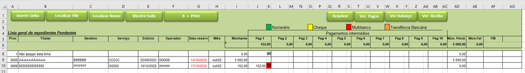
Sub Add_row()
'
' Macro2 Macro
'
'
Application.ScreenUpdating = False
Dim nextrow As Integer
nextrow = Range("A4").End(xlDown).Row
maxfolhas = Application.WorksheetFunction.Max(Sheets("Folha1").Range("A4:A" & nextrow), Sheets("Folha3").Range("A4:A" & Sheets("Folha3").Range("A4").End(xlDown).Row))
Range("A" & nextrow + 1).Value = maxfolhas + 1
Sheets("Folha1").Range("A8:AH8").Select
Selection.Copy
Range("A" & nextrow + 1).Select
Selection.PasteSpecial Paste:=xlPasteFormats, Operation:=xlNone, _
SkipBlanks:=False, Transpose:=False
Application.CutCopyMode = False
Sheets("Folha1").Range("AD8").Select
Selection.Copy
Range("AD" & nextrow + 1).Select
ActiveSheet.Paste
Application.CutCopyMode = False
Sheets("Folha1").Range("AF8").Select
Selection.Copy
Range("AF" & nextrow + 1).Select
ActiveSheet.Paste
Application.CutCopyMode = False
Application.ScreenUpdating = True
End Sub
Sub Delete_filter()
Selection.AutoFilter
End Sub
[CODE=vba]
Sub refresh()
'
' Macro3 Macro
'
Application.ScreenUpdating = False
y = Sheets("Folha1").Range("A7").End(xlDown).Row
For i = 7 To y
DoEvents
x = Sheets("Folha3").Range("A4").End(xlDown).Row + 1
If Sheets("Folha1").Range("AD" & i).Value = 0 And Sheets("Folha1").Range("AE" & i).Value <> 0 Then
Sheets("Folha3").Range("A" & x & ":AH" & x).Value = Sheets("Folha1").Range("A" & i & ":AH" & i).Value
Sheets("Folha3").Select
Range("A7:AH7").Select
Selection.Copy
Sheets("Folha3").Range("A" & x).Select
Selection.PasteSpecial Paste:=xlPasteFormats, Operation:=xlNone, _
SkipBlanks:=False, Transpose:=False
Application.CutCopyMode = False
Sheets("Folha1").Select
Range("AD7").Select
Selection.Copy
Sheets("Folha3").Select
Range("AD" & x).Select
ActiveSheet.Paste
Application.CutCopyMode = False
Sheets("Folha1").Select
Range("AF7").Select
Selection.Copy
Sheets("Folha3").Select
Range("AF" & x).Select
ActiveSheet.Paste
Application.CutCopyMode = False
End If
Next i
Firstrow = 7
LastRow = y
For Lr = LastRow To Firstrow Step -1
With Sheets("Folha1").Cells(Lr, "AD")
If .Value = "0" And .Offset(0, 1) <> 0 Then .EntireRow.Delete
End With
Next Lr
x = Sheets("Folha3").Range("A4").End(xlDown).Row
ActiveWorkbook.Worksheets("Folha3").sort.SortFields.Clear
ActiveWorkbook.Worksheets("Folha3").sort.SortFields.Add Key:=Range("A7"), _
SortOn:=xlSortOnValues, Order:=xlAscending, DataOption:=xlSortNormal
With ActiveWorkbook.Worksheets("Folha3").sort
.SetRange Range("A7:AH" & x)
.Header = xlNo
.MatchCase = False
.Orientation = xlTopToBottom
.SortMethod = xlPinYin
.Apply
End With
Application.ScreenUpdating = False
End Sub