Color scale for above/below average conditional formatting

[kdorClintR]

Is it possible to create a 2-color scale for both below and above average conditional formatting? I'm looking at multiple sets of stats and trying to find where those numbers are both below and above average for that set, but would like to create a color scale so I can visualize how far below or above average those specific numbers are.
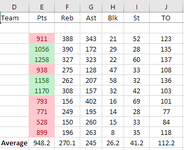
As an example, I would like to see all all cells shaded from red to yellow to green with the lowest number being red, average being yellow, and all numbers above average for that set showing in shades of green. I've tried setting two rules for the specific set of data using above average and below average, but only being able to use one color doesn't really help me visualize how far above or below average the numbers are. Is there a way to do this?

 

[Fluff]

Why not use a 3 colour scale

Fluff.xlsm
	E
1
2
3	911
4	1056
5	1258
6	938
7	1158
8	1170
9	793
10	771
11	528
12	899
13	948.2
14
Main

Cell Formulas
Range	Formula
E13	E13	=AVERAGE(E3:E12)

Cells with Conditional Formatting
Cell	Condition		Cell Format	Stop If True
E3:E12	Other Type	Color scale		NO

 

[kdorClintR]

Why not use a 3 colour scale

Fluff.xlsm
	E
1
2
3	911
4	1056
5	1258
6	938
7	1158
8	1170
9	793
10	771
11	528
12	899
13	948.2
14
Main

Cell Formulas
Range	Formula
E13	E13	=AVERAGE(E3:E12)

Cells with Conditional Formatting
Cell	Condition		Cell Format	Stop If True
E3:E12	Other Type	Color scale		NO

I've considered it, but it doesn't quite give me what I'm looking for. In using a 3-color scale, yellow would represent the median, but not the average. Is there a way to set the 3-color scale so that the yellow would correspond to a set number? That would also work.

 

[Fluff]

You can edit the rule to change the mid point & either use a namer or a formula.

 

[kdorClintR]

I totally skipped over the fact that I could just set the midpoint color to the number representing the average for that dataset. Not the fastest process for 156 datasets, but it will work. Thanks!

 

[Fluff]

Glad to help & thanks for the feedback.