Combination of ISERROR and ISNUMBER in a formula

[meami111]

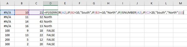
Hi, I am trying to put a formula with a combination of ISERROR and ISNUMBER as follows:
=IF(ISERROR(A2),IF(B2<10,"South",IF(B2>=10,"North",IF(ISNUMBER(A2),IF(C2<20,"South","North")

Getting result for the error values but not for the number values. Seems some issue in the logic. Solicit your help in resolving this

Regards
Amiya C

 

[jasonb75]

See if this works. There are holes in the logic that you could fall through (one that I've noticed). You make no allowance for A2 being text. This is where I have added the text, "Failed" into the formula.

=IF(ISERROR(A2),IF(B2<10,"South","North"),IF(ISNUMBER(A2),IF(C2<20,"South","North"),"Failed"))

 

[meami111]

See if this works. There are holes in the logic that you could fall through (one that I've noticed). You make no allowance for A2 being text. This is where I have added the text, "Failed" into the formula.

=IF(ISERROR(A2),IF(B2<10,"South","North"),IF(ISNUMBER(A2),IF(C2<20,"South","North"),"Failed"))

The column A does not have a text. But can you suggest why the formula is failing for numbers and what should be the solution?

 

[jasonb75]

an you suggest why the formula is failing for numbers

You used too many IF's, the first one had no result for FALSE. The formula would never reach ISNUMBER because of the way it was written.

can you suggest ... what should be the solution?

I already have.

 

[meami111]

You used too many IF's, the first one had no result for FALSE. The formula would never reach ISNUMBER because of the way it was written.

I already have.

Hi Jason
Thanks for your earlier response. I need some more help in this:

How to add a few more nested functions inside and still get a valid answer. Apparently I am getting stuck if more than one nested function is added:
e.g:
=IF(ISERROR(A2),IF(B2<10,"South",IF(B2<20,"West",IF(B2<30,"East","North"),IF(ISNUMBER(A2),IF(C2<20,"South",IF(C2<30,"West",C2<40,"East","North"),"Failed"))

Looking forward to your suggestion

 

[jasonb75]

You're missing a closing bracket in the first section. The 2 IF's that I've marked are both specific to the ISERROR section, so both need to be closed before the next part starts.
Similarly, there are 2 brackets missing in front of "Failed" that relate to the ISNUMBER section.

=IF(ISERROR(A2),IF(B2<10,"South",IF(B2<20,"West",IF(B2<30,"East","North")),IF(ISNUMBER(A2),IF(C2<20,"South",IF(C2<30,"West",IF(C2<40,"East","North"))),"Failed"))

Usually there are better ways than lots of IF's, but remember we can only give answers as good as your questions. While it is a good idea to simplify things when you post, cutting it down too much may not always get you the best help.

This is what I see in your formula, but it may not be what you need.

=LOOKUP(IF(ISERROR(A2),B2+10,C2),{0,20,30,40},{"South","West","East","North"})